Note
Last update 21/07/2021
Application: implementation of existing conceptual models
This page describes the SuperflexPy implementation of several existing conceptual hydrological models. The “translation” of a model into SuperflexPy requires the following steps:
Design of a structure that reflects the original model but satisfies the requirements of SuperflexPy (e.g. does not contain mutual interaction between elements, see Unit);
Extension of the framework, coding the required elements (as explained in the page Expand SuperflexPy: Build customized elements)
Construction of the model structure using the elements implemented at step 2
Model M4 from Kavetski and Fenicia, WRR, 2011
M4 is a simple lumped conceptual model presented, as part of a model comparison study, in the article
Kavetski, D., and F. Fenicia (2011), Elements of a flexible approach for conceptual hydrological modeling: 2. Application and experimental insights, WaterResour.Res.,47, W11511, doi:10.1029/2011WR010748.
Design of the model structure
M4 has a simple structure that can be implemented in SuperflexPy without using connection elements. The figure shows, on the left, the structure as presented in the original M4 publication; on the right, a schematic of the SuperflexPy implementation is shown.
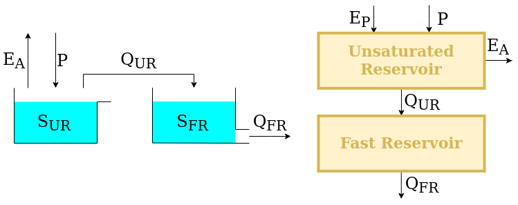
The upstream element, namely, the unsaturated reservoir (UR), is intended to represent runoff generation processes (e.g. separation between evaporation and runoff). It is controlled by the differential equation
The downstream element, namely, the fast reservoir (FR), is intended to represent runoff propagation processes (e.g. routing). It is controlled by the differential equation
\(S_{\textrm{UR}}\) and \(S_{\textrm{FR}}\) are the model states, \(P\) is the precipitation input flux, \(E_{\textrm{P}}\) is the potential evapotranspiration (a model input), and \(S_{\textrm{max}}\), \(m\), \(\beta\), \(k\), \(\alpha\) are the model parameters.
Element creation
We now show how to use SuperflexPy to implement the elements described in the previous section. A detailed explanation of how to use the framework to build new elements can be found in the page Expand SuperflexPy: Build customized elements.
Note that, most of the times, when implementing a model structure with SuperflexPym the elements have already been implemented in SuperflexPy and, therefore, the modeller does not need to implement them. A list of the currently implemented elements is provided in the page List of currently implemented elements.
Unsaturated reservoir
This element can be implemented by extending the class ODEsElement.
  1class UnsaturatedReservoir(ODEsElement):
  2
  3    def __init__(self, parameters, states, approximation, id):
  4
  5        ODEsElement.__init__(self,
  6                             parameters=parameters,
  7                             states=states,
  8                             approximation=approximation,
  9                             id=id)
 10
 11        self._fluxes_python = [self._fluxes_function_python]
 12
 13        if approximation.architecture == 'numba':
 14            self._fluxes = [self._fluxes_function_numba]
 15        elif approximation.architecture == 'python':
 16            self._fluxes = [self._fluxes_function_python]
 17
 18    def set_input(self, input):
 19
 20        self.input = {'P': input[0],
 21                      'PET': input[1]}
 22
 23    def get_output(self, solve=True):
 24
 25        if solve:
 26            self._solver_states = [self._states[self._prefix_states + 'S0']]
 27
 28            self._solve_differential_equation()
 29
 30            # Update the state
 31            self.set_states({self._prefix_states + 'S0': self.state_array[-1, 0]})
 32
 33        fluxes = self._num_app.get_fluxes(fluxes=self._fluxes_python,
 34                                          S=self.state_array,
 35                                          S0=self._solver_states,
 36                                          dt=self._dt,
 37                                          **self.input,
 38                                          **{k[len(self._prefix_parameters):]: self._parameters[k] for k in self._parameters},
 39                                          )
 40        return [-fluxes[0][2]]
 41
 42    def get_AET(self):
 43
 44        try:
 45            S = self.state_array
 46        except AttributeError:
 47            message = '{}get_aet method has to be run after running '.format(self._error_message)
 48            message += 'the model using the method get_output'
 49            raise AttributeError(message)
 50
 51        fluxes = self._num_app.get_fluxes(fluxes=self._fluxes_python,
 52                                          S=S,
 53                                          S0=self._solver_states,
 54                                          dt=self._dt,
 55                                          **self.input,
 56                                          **{k[len(self._prefix_parameters):]: self._parameters[k] for k in self._parameters},
 57                                          )
 58        return [- fluxes[0][1]]
 59
 60    # PROTECTED METHODS
 61
 62    @staticmethod
 63    def _fluxes_function_python(S, S0, ind, P, Smax, m, beta, PET, dt):
 64
 65        if ind is None:
 66            return (
 67                [
 68                    P,
 69                    - PET * ((S / Smax) * (1 + m)) / ((S / Smax) + m),
 70                    - P * (S / Smax)**beta,
 71                ],
 72                0.0,
 73                S0 + P * dt
 74            )
 75        else:
 76            return (
 77                [
 78                    P[ind],
 79                    - PET[ind] * ((S / Smax[ind]) * (1 + m[ind])) / ((S / Smax[ind]) + m[ind]),
 80                    - P[ind] * (S / Smax[ind])**beta[ind],
 81                ],
 82                0.0,
 83                S0 + P[ind] * dt[ind],
 84                [
 85                    0.0,
 86                    - (Ce[ind] * PET[ind] * m[ind] * (m[ind] + 1) * Smax[ind])/((S + m[ind] * Smax[ind])**2),
 87                    - (P[ind] * beta[ind] / Smax[ind]) * (S / Smax[ind])**(beta[ind] - 1),
 88                ]
 89            )
 90
 91    @staticmethod
 92    @nb.jit('Tuple((UniTuple(f8, 3), f8, f8, UniTuple(f8, 3)))(optional(f8), f8, i4, f8[:], f8[:], f8[:], f8[:], f8[:], f8[:])',
 93            nopython=True)
 94    def _fluxes_function_numba(S, S0, ind, P, Smax, m, beta, PET, dt):
 95
 96        return (
 97            (
 98                P[ind],
 99                PET[ind] * ((S / Smax[ind]) * (1 + m[ind])) / ((S / Smax[ind]) + m[ind]),
100                - P[ind] * (S / Smax[ind])**beta[ind],
101            ),
102            0.0,
103            S0 + P[ind] * dt[ind],
104            (
105                0.0,
106                - (Ce[ind] * PET[ind] * m[ind] * (m[ind] + 1) * Smax[ind])/((S + m[ind] * Smax[ind])**2),
107                - (P[ind] * beta[ind] / Smax[ind]) * (S / Smax[ind])**(beta[ind] - 1),
108            )
109        )
Fast reservoir
This element can be implemented by extending the class ODEsElement.
 1class PowerReservoir(ODEsElement):
 2
 3    def __init__(self, parameters, states, approximation, id):
 4
 5        ODEsElement.__init__(self,
 6                             parameters=parameters,
 7                             states=states,
 8                             approximation=approximation,
 9                             id=id)
10
11        self._fluxes_python = [self._fluxes_function_python]  # Used by get fluxes, regardless of the architecture
12
13        if approximation.architecture == 'numba':
14            self._fluxes = [self._fluxes_function_numba]
15        elif approximation.architecture == 'python':
16            self._fluxes = [self._fluxes_function_python]
17
18    # METHODS FOR THE USER
19
20    def set_input(self, input):
21
22        self.input = {'P': input[0]}
23
24    def get_output(self, solve=True):
25
26        if solve:
27            self._solver_states = [self._states[self._prefix_states + 'S0']]
28            self._solve_differential_equation()
29
30            # Update the state
31            self.set_states({self._prefix_states + 'S0': self.state_array[-1, 0]})
32
33        fluxes = self._num_app.get_fluxes(fluxes=self._fluxes_python,  # I can use the python method since it is fast
34                                          S=self.state_array,
35                                          S0=self._solver_states,
36                                          dt=self._dt,
37                                          **self.input,
38                                          **{k[len(self._prefix_parameters):]: self._parameters[k] for k in self._parameters},
39                                          )
40
41        return [- fluxes[0][1]]
42
43    # PROTECTED METHODS
44
45    @staticmethod
46    def _fluxes_function_python(S, S0, ind, P, k, alpha, dt):
47
48        if ind is None:
49            return (
50                [
51                    P,
52                    - k * S**alpha,
53                ],
54                0.0,
55                S0 + P * dt
56            )
57        else:
58            return (
59                [
60                    P[ind],
61                    - k[ind] * S**alpha[ind],
62                ],
63                0.0,
64                S0 + P[ind] * dt[ind],
65                [
66                    0.0,
67                    - k[ind] * alpha[ind] * S**(alpha[ind] - 1)
68                ]
69            )
70
71    @staticmethod
72    @nb.jit('Tuple((UniTuple(f8, 2), f8, f8, UniTuple(f8, 2)))(optional(f8), f8, i4, f8[:], f8[:], f8[:], f8[:])',
73            nopython=True)
74    def _fluxes_function_numba(S, S0, ind, P, k, alpha, dt):
75
76        return (
77            (
78                P[ind],
79                - k[ind] * S**alpha[ind],
80            ),
81            0.0,
82            S0 + P[ind] * dt[ind],
83            (
84                0.0,
85                - k[ind] * alpha[ind] * S**(alpha[ind] - 1)
86            )
87        )
Model initialization
Now that all elements are implemented, they can be combined to build the model structure. For details refer to How to build a model with SuperflexPy.
First, we initialize all elements.
 1root_finder = PegasusPython()
 2numeric_approximator = ImplicitEulerPython(root_finder=root_finder)
 3
 4ur = UnsaturatedReservoir(
 5    parameters={'Smax': 50.0, 'Ce': 1.0, 'm': 0.01, 'beta': 2.0},
 6    states={'S0': 25.0},
 7    approximation=numeric_approximator,
 8    id='UR'
 9)
10
11fr = PowerReservoir(
12    parameters={'k': 0.1, 'alpha': 1.0},
13    states={'S0': 10.0},
14    approximation=numeric_approximator,
15    id='FR'
16)
Next, the elements can be put together to create a Unit that reflects
the structure presented in the figure.
1model = Unit(
2    layers=[
3        [ur],
4        [fr]
5    ],
6    id='M4'
GR4J
GR4J is a widely used conceptual hydrological model introduced in the article
Perrin, C., Michel, C., and Andréassian, V.: Improvement of a parsimonious model for streamflow simulation, Journal of Hydrology, 279, 275-289, https://doi.org/10.1016/S0022-1694(03)00225-7, 2003.
The solution adopted here follows the “continuous state-space representation” presented in
Santos, L., Thirel, G., and Perrin, C.: Continuous state-space representation of a bucket-type rainfall-runoff model: a case study with the GR4 model using state-space GR4 (version 1.0), Geosci. Model Dev., 11, 1591-1605, 10.5194/gmd-11-1591-2018, 2018.
Design of the model structure
The figure shows, on the left, the model structure as presented in Perrin et al., 2003; on the right, the adaptation to SuperflexPy is shown.
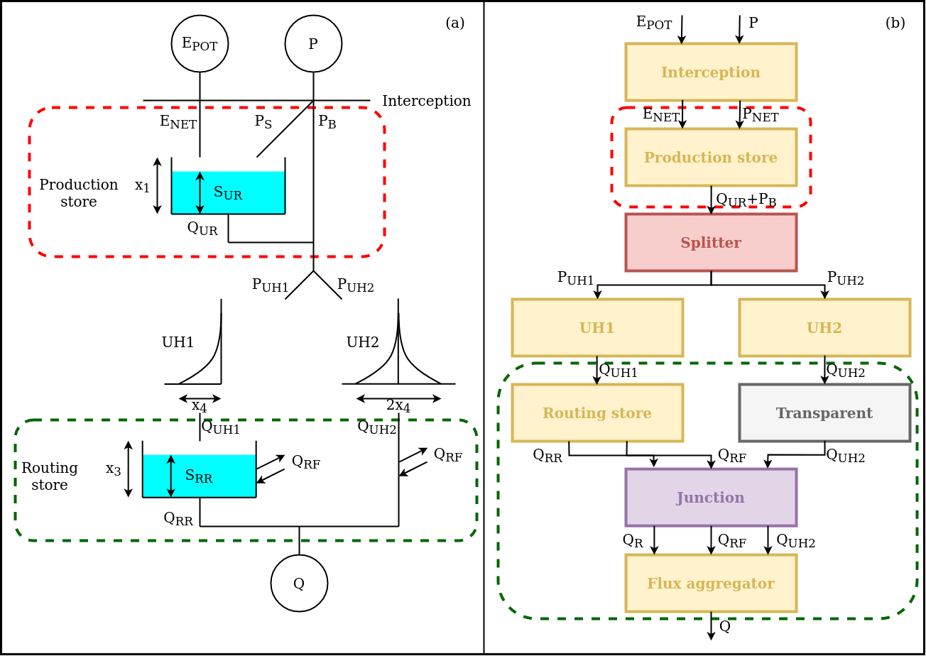
The potential evaporation and the precipitation are “filtered” by an interception element, that calculates the net fluxes by setting the smallest to zero and the largest to the difference between the two fluxes.
This element is implemented in SuperflexPy using the “interception filter”.
After the interception filter, the SuperflexPy implementation starts to differ from the original. In the original implementation of GR4J, the precipitation is split between a part \(P_{\textrm{s}}\) that flows into the production store and the remaining part \(P_{\textrm{b}}\) that bypasses the reservoir. \(P_{\textrm{s}}\) and \(P_{\textrm{b}}\) are both functions of the state of the reservoir
When we implement this part of the model in SuperflexPy, these two fluxes cannot be calculated before solving the reservoir (due to the representation of the Unit as a succession of layers).
To solve this problem, in the SuperflexPy implementation of GR4J, all precipitation (and not only \(P_{\textrm{s}}\)) flows into an element that incorporates the production store. This element takes care of dividing the precipitation internally, while solving the differential equation
where the first term is the precipitation \(P_s\), the second term is the actual evaporation, and the third term represents the output of the reservoir, which here corresponds to “percolation”.
Once the reservoir is solved (i.e. the values of \(S_{\textrm{UR}}\) that solve the discretized differential equation over a time step are found), the element outputs the sum of percolation and bypassing precipitation (\(P_b\)).
The flux is then divided between two lag functions, referred to as “unit hydrographs” and abbreviated UH: 90% of the flux goes to UH1 and 10% goes to UH2. In this part of the model structure the correspondence between the elements of GR4J and their SuperflexPy implementation is quite clear.
The output of UH1 provides the input of the routing store, which is a reservoir controlled by the differential equation
where the second term is the output of the reservoir and the last is a gain/loss term (called \(Q_{\textrm{RF}}\)).
The gain/loss term \(Q_{\textrm{RF}}\), which is a function of the state \(S_{\textrm{RR}}\) of the reservoir, is also subtracted from the output of UH2. In SuperflexPy, this operation cannot be done in the same unit layer as the solution of the routing store, and instead it is done afterwards. For this reason, the SuperflexPy implementation of GR4J has an additional element (called “flux aggregator”) that uses a junction element to combine the output of the routing store, the gain/loss term, and the output of UH2. The flux aggregator then computes the outflow of the model using the equation
Elements creation
We now show how to use SuperflexPy to implement the elements described in the previous section. A detailed explanation of how to use the framework to build new elements can be found in the page Expand SuperflexPy: Build customized elements.
Note that, most of the times, when implementing a model structure with SuperflexPym the elements have already been implemented in SuperflexPy and, therefore, the modeller does not need to implement them. A list of the currently implemented elements is provided in the page List of currently implemented elements.
Interception
The interception filter can be implemented by extending the class
BaseElement
 1class InterceptionFilter(BaseElement):
 2
 3    _num_upstream = 1
 4    _num_downstream = 1
 5
 6    def set_input(self, input):
 7
 8        self.input = {}
 9        self.input['PET'] = input[0]
10        self.input['P'] = input[1]
11
12    def get_output(self, solve=True):
13
14        remove = np.minimum(self.input['PET'], self.input['P'])
15
16        return [self.input['PET'] - remove, self.input['P'] - remove]
Production store
The production store is controlled by a differential equation and, therefore,
can be constructed by extending the class ODEsElement
  1class ProductionStore(ODEsElement):
  2
  3    def __init__(self, parameters, states, approximation, id):
  4
  5        ODEsElement.__init__(self,
  6                             parameters=parameters,
  7                             states=states,
  8                             approximation=approximation,
  9                             id=id)
 10
 11        self._fluxes_python = [self._flux_function_python]
 12
 13        if approximation.architecture == 'numba':
 14            self._fluxes = [self._flux_function_numba]
 15        elif approximation.architecture == 'python':
 16            self._fluxes = [self._flux_function_python]
 17
 18    def set_input(self, input):
 19
 20        self.input = {}
 21        self.input['PET'] = input[0]
 22        self.input['P'] = input[1]
 23
 24    def get_output(self, solve=True):
 25
 26        if solve:
 27            # Solve the differential equation
 28            self._solver_states = [self._states[self._prefix_states + 'S0']]
 29            self._solve_differential_equation()
 30
 31            # Update the states
 32            self.set_states({self._prefix_states + 'S0': self.state_array[-1, 0]})
 33
 34        fluxes = self._num_app.get_fluxes(fluxes=self._fluxes_python,
 35                                          S=self.state_array,
 36                                          S0=self._solver_states,
 37                                          dt=self._dt,
 38                                          **self.input,
 39                                          **{k[len(self._prefix_parameters):]: self._parameters[k] for k in self._parameters},
 40                                          )
 41
 42        Pn_minus_Ps = self.input['P'] - fluxes[0][0]
 43        Perc = - fluxes[0][2]
 44        return [Pn_minus_Ps + Perc]
 45
 46    def get_aet(self):
 47
 48        try:
 49            S = self.state_array
 50        except AttributeError:
 51            message = '{}get_aet method has to be run after running '.format(self._error_message)
 52            message += 'the model using the method get_output'
 53            raise AttributeError(message)
 54
 55        fluxes = self._num_app.get_fluxes(fluxes=self._fluxes_python,
 56                                          S=S,
 57                                          S0=self._solver_states,
 58                                          dt=self._dt,
 59                                          **self.input,
 60                                          **{k[len(self._prefix_parameters):]: self._parameters[k] for k in self._parameters},
 61                                          )
 62
 63        return [- fluxes[0][1]]
 64
 65    @staticmethod
 66    def _flux_function_python(S, S0, ind, P, x1, alpha, beta, ni, PET, dt):
 67
 68        if ind is None:
 69            return(
 70                [
 71                    P * (1 - (S / x1)**alpha),  # Ps
 72                    - PET * (2 * (S / x1) - (S / x1)**alpha),  # Evaporation
 73                    - ((x1**(1 - beta)) / ((beta - 1))) * (ni**(beta - 1)) * (S**beta)  # Perc
 74                ],
 75                0.0,
 76                S0 + P * (1 - (S / x1)**alpha) * dt
 77            )
 78        else:
 79            return(
 80                [
 81                    P[ind] * (1 - (S / x1[ind])**alpha[ind]),  # Ps
 82                    - PET[ind] * (2 * (S / x1[ind]) - (S / x1[ind])**alpha[ind]),  # Evaporation
 83                    - ((x1[ind]**(1 - beta[ind])) / ((beta[ind] - 1))) * (ni[ind]**(beta[ind] - 1)) * (S**beta[ind])  # Perc
 84                ],
 85                0.0,
 86                S0 + P[ind] * (1 - (S / x1[ind])**alpha[ind]) * dt[ind],
 87                [
 88                    - (P[ind] * alpha[ind] / x1[ind]) * ((S / x1[ind])**(alpha[ind] - 1)),
 89                    - (PET[ind] / x1[ind]) * (2 - alpha[ind] * ((S / x1[ind])**(alpha[ind] - 1))),
 90                    - beta[ind] * ((x1[ind]**(1 - beta[ind])) / ((beta[ind] - 1) * dt[ind])) * (ni[ind]**(beta[ind] - 1)) * (S**(beta[ind] - 1))
 91                ]
 92            )
 93
 94    @staticmethod
 95    @nb.jit('Tuple((UniTuple(f8, 3), f8, f8, UniTuple(f8, 3)))(optional(f8), f8, i4, f8[:], f8[:], f8[:], f8[:], f8[:], f8[:], f8[:])',
 96            nopython=True)
 97    def _flux_function_numba(S, S0, ind, P, x1, alpha, beta, ni, PET, dt):
 98
 99        return(
100            (
101                P[ind] * (1 - (S / x1[ind])**alpha[ind]),  # Ps
102                - PET[ind] * (2 * (S / x1[ind]) - (S / x1[ind])**alpha[ind]),  # Evaporation
103                - ((x1[ind]**(1 - beta[ind])) / ((beta[ind] - 1))) * (ni[ind]**(beta[ind] - 1)) * (S**beta[ind])  # Perc
104            ),
105            0.0,
106            S0 + P[ind] * (1 - (S / x1[ind])**alpha[ind]) * dt[ind],
107            (
108                - (P[ind] * alpha[ind] / x1[ind]) * ((S / x1[ind])**(alpha[ind] - 1)),
109                - (PET[ind] / x1[ind]) * (2 - alpha[ind] * ((S / x1[ind])**(alpha[ind] - 1))),
110                - beta[ind] * ((x1[ind]**(1 - beta[ind])) / ((beta[ind] - 1) * dt[ind])) * (ni[ind]**(beta[ind] - 1)) * (S**(beta[ind] - 1))
111            )
112        )
Unit hydrographs
The unit hydrographs are an extension of the LagElement, and can be
implemented as follows
 1class UnitHydrograph1(LagElement):
 2
 3    def __init__(self, parameters, states, id):
 4
 5        LagElement.__init__(self, parameters, states, id)
 6
 7    def _build_weight(self, lag_time):
 8
 9        weight = []
10
11        for t in lag_time:
12            array_length = np.ceil(t)
13            w_i = []
14            for i in range(int(array_length)):
15                w_i.append(self._calculate_lag_area(i + 1, t)
16                           - self._calculate_lag_area(i, t))
17            weight.append(np.array(w_i))
18
19        return weight
20
21    @staticmethod
22    def _calculate_lag_area(bin, len):
23        if bin <= 0:
24            value = 0
25        elif bin < len:
26            value = (bin / len)**2.5
27        else:
28            value = 1
29        return value
 1class UnitHydrograph2(LagElement):
 2
 3    def __init__(self, parameters, states, id):
 4
 5        LagElement.__init__(self, parameters, states, id)
 6
 7    def _build_weight(self, lag_time):
 8
 9        weight = []
10
11        for t in lag_time:
12            array_length = np.ceil(t)
13            w_i = []
14            for i in range(int(array_length)):
15                w_i.append(self._calculate_lag_area(i + 1, t)
16                           - self._calculate_lag_area(i, t))
17            weight.append(np.array(w_i))
18
19        return weight
20
21    @staticmethod
22    def _calculate_lag_area(bin, len):
23        half_len = len / 2
24        if bin <= 0:
25            value = 0
26        elif bin < half_len:
27            value = 0.5 * (bin / half_len)**2.5
28        elif bin < len:
29            value = 1 - 0.5 * (2 - bin / half_len)**2.5
30        else:
31            value = 1
32        return value
Routing store
The routing store is an ODEsElement
 1class RoutingStore(ODEsElement):
 2
 3    def __init__(self, parameters, states, approximation, id):
 4
 5        ODEsElement.__init__(self,
 6                             parameters=parameters,
 7                             states=states,
 8                             approximation=approximation,
 9                             id=id)
10
11        self._fluxes_python = [self._flux_function_python]
12
13        if approximation.architecture == 'numba':
14            self._fluxes = [self._flux_function_numba]
15        elif approximation.architecture == 'python':
16            self._fluxes = [self._flux_function_python]
17
18    def set_input(self, input):
19
20        self.input = {}
21        self.input['P'] = input[0]
22
23    def get_output(self, solve=True):
24
25        if solve:
26            # Solve the differential equation
27            self._solver_states = [self._states[self._prefix_states + 'S0']]
28            self._solve_differential_equation()
29
30            # Update the states
31            self.set_states({self._prefix_states + 'S0': self.state_array[-1, 0]})
32
33        fluxes = self._num_app.get_fluxes(fluxes=self._fluxes_python,
34                                          S=self.state_array,
35                                          S0=self._solver_states,
36                                          dt=self._dt,
37                                          **self.input,
38                                          **{k[len(self._prefix_parameters):]: self._parameters[k] for k in self._parameters},
39                                          )
40
41        Qr = - fluxes[0][1]
42        F = -fluxes[0][2]
43
44        return [Qr, F]
45
46    @staticmethod
47    def _flux_function_python(S, S0, ind, P, x2, x3, gamma, omega, dt):
48
49        if ind is None:
50            return(
51                [
52                    P,  # P
53                    - ((x3**(1 - gamma)) / ((gamma - 1))) * (S**gamma),  # Qr
54                    - (x2 * (S / x3)**omega),  # F
55                ],
56                0.0,
57                S0 + P * dt
58            )
59        else:
60            return(
61                [
62                    P[ind],  # P
63                    - ((x3[ind]**(1 - gamma[ind])) / ((gamma[ind] - 1))) * (S**gamma[ind]),  # Qr
64                    - (x2[ind] * (S / x3[ind])**omega[ind]),  # F
65                ],
66                0.0,
67                S0 + P[ind] * dt[ind],
68                [
69                    0.0,
70                    - ((x3[ind]**(1 - gamma[ind])) / ((gamma[ind] - 1) * dt[ind])) * (S**(gamma[ind] - 1)) * gamma[ind],
71                    - (omega[ind] * x2[ind] * ((S / x3[ind])**(omega[ind] - 1)))
72                ]
73            )
74
75    @staticmethod
76    @nb.jit('Tuple((UniTuple(f8, 3), f8, f8, UniTuple(f8, 3)))(optional(f8), f8, i4, f8[:], f8[:], f8[:], f8[:], f8[:], f8[:])',
77            nopython=True)
78    def _flux_function_numba(S, S0, ind, P, x2, x3, gamma, omega, dt):
79
80        return(
81            (
82                P[ind],  # P
83                - ((x3[ind]**(1 - gamma[ind])) / ((gamma[ind] - 1))) * (S**gamma[ind]),  # Qr
84                - (x2[ind] * (S / x3[ind])**omega[ind]),  # F
85            ),
86            0.0,
87            S0 + P[ind] * dt[ind],
88            (
89                0.0,
90                - ((x3[ind]**(1 - gamma[ind])) / ((gamma[ind] - 1) * dt[ind])) * (S**(gamma[ind] - 1)) * gamma[ind],
91                - (omega[ind] * x2[ind] * ((S / x3[ind])**(omega[ind] - 1)))
92            )
93        )
Flux aggregator
The flux aggregator can be implemented by extending a BaseElement
 1class FluxAggregator(BaseElement):
 2
 3    _num_downstream = 1
 4    _num_upstream = 1
 5
 6    def set_input(self, input):
 7
 8        self.input = {}
 9        self.input['Qr'] = input[0]
10        self.input['F'] = input[1]
11        self.input['Q2_out'] = input[2]
12
13    def get_output(self, solve=True):
14
15        return [self.input['Qr']
16                + np.maximum(0, self.input['Q2_out'] - self.input['F'])]
Model initialization
Now that all elements are implemented, we can combine them to build the model structure. For details refer to How to build a model with SuperflexPy.
First, we initialize all elements.
 1x1, x2, x3, x4 = (50.0, 0.1, 20.0, 3.5)
 2
 3root_finder = PegasusPython()  # Use the default parameters
 4numerical_approximation = ImplicitEulerPython(root_finder)
 5
 6interception_filter = InterceptionFilter(id='ir')
 7
 8production_store = ProductionStore(parameters={'x1': x1, 'alpha': 2.0,
 9                                               'beta': 5.0, 'ni': 4/9},
10                                   states={'S0': 10.0},
11                                   approximation=numerical_approximation,
12                                   id='ps')
13
14splitter = Splitter(weight=[[0.9], [0.1]],
15                    direction=[[0], [0]],
16                    id='spl')
17
18unit_hydrograph_1 = UnitHydrograph1(parameters={'lag-time': x4},
19                                    states={'lag': None},
20                                    id='uh1')
21
22unit_hydrograph_2 = UnitHydrograph2(parameters={'lag-time': 2*x4},
23                                    states={'lag': None},
24                                    id='uh2')
25
26routing_store = RoutingStore(parameters={'x2': x2, 'x3': x3,
27                                         'gamma': 5.0, 'omega': 3.5},
28                             states={'S0': 10.0},
29                             approximation=numerical_approximation,
30                             id='rs')
31
32transparent = Transparent(id='tr')
33
34junction = Junction(direction=[[0, None],  # First output
35                               [1, None],  # Second output
36                               [None, 0]], # Third output
37                    id='jun')
38
39flux_aggregator = FluxAggregator(id='fa')
The elements are then put together to define a Unit that reflects the
GR4J structure presented in the figure.
1model = Unit(layers=[[interception_filter],
2                     [production_store],
3                     [splitter],
4                     [unit_hydrograph_1, unit_hydrograph_2],
5                     [routing_store, transparent],
6                     [junction],
7                     [flux_aggregator]],
8             id='model')
HYMOD
HYMOD is another widely used conceptual hydrological model. It was first published in
Boyle, D. P. (2001). Multicriteria calibration of hydrologic models, The University of Arizona. Link
The solution proposed here follows the model structure presented in
Wagener, T., Boyle, D. P., Lees, M. J., Wheater, H. S., Gupta, H. V., and Sorooshian, S.: A framework for development and application of hydrological models, Hydrol. Earth Syst. Sci., 5, 13–26, https://doi.org/10.5194/hess-5-13-2001, 2001.
Design of the structure
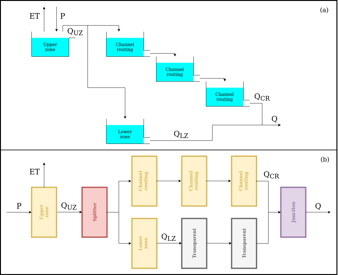
HYMOD comprises three groups of reservoirs intended to represent, respectively, the upper zone (soil dynamics), channel routing (surface runoff), and lower zone (subsurface flow).
As can be seen in the figure, the original structure of HYMOD already meets the design constrains of SuperflexPy (it does not contains feedbacks between elements). Therefore the SuperflexPy implementation of HYMOD is more straightforward than for GR4J.
The upper zone is a reservoir intended to represent streamflow generation processes and evaporation. It is controlled by the differential equation
where the first term is the precipitation input, the second term is the actual evaporation (which is equal to the potential evaporation as long as there is sufficient storage in the reservoir), and the third term is the outflow from the reservoir.
The outflow from the reservoir is then split between the channel routing (3 reservoirs) and the lower zone (1 reservoir). All these elements are represented by linear reservoirs controlled by the differential equation
where the first term is the input (here, the outflow from the upstream element) and the second term represents the outflow from the reservoir.
Channel routing and lower zone differ from each other in the number of reservoirs used (3 in the first case and 1 in the second), and in the value of the parameter \(k\), which controls the outflow rate. Based on intended model operation, \(k\) should have a larger value for channel routing because this element is intended to represent faster processes.
The outputs of these two flowpaths are collected by a junction, which generates the final model output.
Comparing the two panels in the figure, the only difference is the presence of the two transparent elements that are needed to fill the “gaps” in the SuperflexPy structure (see Unit).
Elements creation
We now show how to use SuperflexPy to implement the elements described in the previous section. A detailed explanation of how to use the framework to build new elements can be found in the page Expand SuperflexPy: Build customized elements.
Note that, most of the times, when implementing a model structure with SuperflexPym the elements have already been implemented in SuperflexPy and, therefore, the modeller does not need to implement them. A list of the currently implemented elements is provided in the page List of currently implemented elements.
Upper zone
The code used to simulate the upper zone present a change in the equation used to calculate the actual evaporation. In the original version (Wagener et al., 1) the equation is “described” in the text
The actual evapotranspiration is equal to the potential value if sufficient soil moisture is available; otherwise it is equal to the available soil moisture content.
which translates to the equation
Note that this solution is not smooth and the resulting sharp threshold can cause problematic discontinuities in the model behavior. A smooth version of this equation is given by
The upper zone reservoir can be implemented by extending the class
ODEsElement.
  1class UpperZone(ODEsElement):
  2
  3    def __init__(self, parameters, states, approximation, id):
  4
  5        ODEsElement.__init__(self,
  6                             parameters=parameters,
  7                             states=states,
  8                             approximation=approximation,
  9                             id=id)
 10
 11        self._fluxes_python = [self._fluxes_function_python]
 12
 13        if approximation.architecture == 'numba':
 14            self._fluxes = [self._fluxes_function_numba]
 15        elif approximation.architecture == 'python':
 16            self._fluxes = [self._fluxes_function_python]
 17
 18    def set_input(self, input):
 19
 20        self.input = {'P': input[0],
 21                      'PET': input[1]}
 22
 23    def get_output(self, solve=True):
 24
 25        if solve:
 26            self._solver_states = [self._states[self._prefix_states + 'S0']]
 27
 28            self._solve_differential_equation()
 29
 30            # Update the state
 31            self.set_states({self._prefix_states + 'S0': self.state_array[-1, 0]})
 32
 33        fluxes = self._num_app.get_fluxes(fluxes=self._fluxes_python,
 34                                          S=self.state_array,
 35                                          S0=self._solver_states,
 36                                          dt=self._dt,
 37                                          **self.input,
 38                                          **{k[len(self._prefix_parameters):]: self._parameters[k] for k in self._parameters},
 39                                          )
 40        return [-fluxes[0][2]]
 41
 42    def get_AET(self):
 43
 44        try:
 45            S = self.state_array
 46        except AttributeError:
 47            message = '{}get_aet method has to be run after running '.format(self._error_message)
 48            message += 'the model using the method get_output'
 49            raise AttributeError(message)
 50
 51        fluxes = self._num_app.get_fluxes(fluxes=self._fluxes_python,
 52                                          S=S,
 53                                          S0=self._solver_states,
 54                                          dt=self._dt,
 55                                          **self.input,
 56                                          **{k[len(self._prefix_parameters):]: self._parameters[k] for k in self._parameters},
 57                                          )
 58        return [- fluxes[0][1]]
 59
 60    # PROTECTED METHODS
 61
 62    @staticmethod
 63    def _fluxes_function_python(S, S0, ind, P, Smax, m, beta, PET, dt):
 64
 65        if ind is None:
 66            return (
 67                [
 68                    P,
 69                    - PET * ((S / Smax) * (1 + m)) / ((S / Smax) + m),
 70                    - P * (1 - (1 - (S / Smax))**beta),
 71                ],
 72                0.0,
 73                S0 + P * dt
 74            )
 75        else:
 76            return (
 77                [
 78                    P[ind],
 79                    - PET[ind] * ((S / Smax[ind]) * (1 + m[ind])) / ((S / Smax[ind]) + m[ind]),
 80                    - P[ind] * (1 - (1 - (S / Smax[ind]))**beta[ind]),
 81                ],
 82                0.0,
 83                S0 + P[ind] * dt[ind],
 84                [
 85                    0.0,
 86                    - PET[ind] * m[ind] * Smax[ind] * (1 + m[ind]) / ((S + Smax[ind] * m[ind])**2),
 87                    - P[ind] * beta[ind] * ((1 - (S / Smax[ind]))**(beta[ind] - 1)) / Smax[ind],
 88                ]
 89            )
 90
 91    @staticmethod
 92    @nb.jit('Tuple((UniTuple(f8, 3), f8, f8, UniTuple(f8, 3)))(optional(f8), f8, i4, f8[:], f8[:], f8[:], f8[:], f8[:], f8[:])',
 93            nopython=True)
 94    def _fluxes_function_numba(S, S0, ind, P, Smax, m, beta, PET, dt):
 95
 96        return (
 97            (
 98                P[ind],
 99                - PET[ind] * ((S / Smax[ind]) * (1 + m[ind])) / ((S / Smax[ind]) + m[ind]),
100                - P[ind] * (1 - (1 - (S / Smax[ind]))**beta[ind]),
101            ),
102            0.0,
103            S0 + P[ind] * dt[ind],
104            (
105                0.0,
106                - PET[ind] * m[ind] * Smax[ind] * (1 + m[ind]) / ((S + Smax[ind] * m[ind])**2),
107                - P[ind] * beta[ind] * ((1 - (S / Smax[ind]))**(beta[ind] - 1)) / Smax[ind],
108            )
109        )
Channel routing and lower zone
The elements representing channel routing and lower zone are all linear
reservoirs that can be implemented by extending the class ODEsElement.
 1class LinearReservoir(ODEsElement):
 2
 3    def __init__(self, parameters, states, approximation, id):
 4
 5        ODEsElement.__init__(self,
 6                             parameters=parameters,
 7                             states=states,
 8                             approximation=approximation,
 9                             id=id)
10
11        self._fluxes_python = [self._fluxes_function_python]  # Used by get fluxes, regardless of the architecture
12
13        if approximation.architecture == 'numba':
14            self._fluxes = [self._fluxes_function_numba]
15        elif approximation.architecture == 'python':
16            self._fluxes = [self._fluxes_function_python]
17
18    # METHODS FOR THE USER
19
20    def set_input(self, input):
21
22        self.input = {'P': input[0]}
23
24    def get_output(self, solve=True):
25
26        if solve:
27            self._solver_states = [self._states[self._prefix_states + 'S0']]
28            self._solve_differential_equation()
29
30            # Update the state
31            self.set_states({self._prefix_states + 'S0': self.state_array[-1, 0]})
32
33        fluxes = self._num_app.get_fluxes(fluxes=self._fluxes_python,  # I can use the python method since it is fast
34                                          S=self.state_array,
35                                          S0=self._solver_states,
36                                          dt=self._dt,
37                                          **self.input,
38                                          **{k[len(self._prefix_parameters):]: self._parameters[k] for k in self._parameters},
39                                          )
40        return [- fluxes[0][1]]
41
42    # PROTECTED METHODS
43
44    @staticmethod
45    def _fluxes_function_python(S, S0, ind, P, k, dt):
46
47        if ind is None:
48            return (
49                [
50                    P,
51                    - k * S,
52                ],
53                0.0,
54                S0 + P * dt
55            )
56        else:
57            return (
58                [
59                    P[ind],
60                    - k[ind] * S,
61                ],
62                0.0,
63                S0 + P[ind] * dt[ind],
64                [
65                    0.0,
66                    - k[ind]
67                ]
68            )
69
70    @staticmethod
71    @nb.jit('Tuple((UniTuple(f8, 2), f8, f8, UniTuple(f8, 2)))(optional(f8), f8, i4, f8[:], f8[:], f8[:])',
72            nopython=True)
73    def _fluxes_function_numba(S, S0, ind, P, k, dt):
74
75        return (
76            (
77                P[ind],
78                - k[ind] * S,
79            ),
80            0.0,
81            S0 + P[ind] * dt[ind],
82            (
83                0.0,
84                - k[ind]
85            )
86        )
Model initialization
Now that all elements are implemented, we can combine them to build the HYMOD model structure. For details refer to How to build a model with SuperflexPy.
First, we initialize all elements.
 1root_finder = PegasusPython()  # Use the default parameters
 2numerical_approximation = ImplicitEulerPython(root_finder)
 3
 4upper_zone = UpperZone(parameters={'Smax': 50.0, 'm': 0.01, 'beta': 2.0},
 5                       states={'S0': 10.0},
 6                       approximation=numerical_approximation,
 7                       id='uz')
 8
 9splitter = Splitter(weight=[[0.6], [0.4]],
10                    direction=[[0], [0]],
11                    id='spl')
12
13channel_routing_1 = LinearReservoir(parameters={'k': 0.1},
14                                    states={'S0': 10.0},
15                                    approximation=numerical_approximation,
16                                    id='cr1')
17
18channel_routing_2 = LinearReservoir(parameters={'k': 0.1},
19                                    states={'S0': 10.0},
20                                    approximation=numerical_approximation,
21                                    id='cr2')
22
23channel_routing_3 = LinearReservoir(parameters={'k': 0.1},
24                                    states={'S0': 10.0},
25                                    approximation=numerical_approximation,
26                                    id='cr3')
27
28lower_zone = LinearReservoir(parameters={'k': 0.1},
29                             states={'S0': 10.0},
30                             approximation=numerical_approximation,
31                             id='lz')
32
33transparent_1 = Transparent(id='tr1')
34
35transparent_2 = Transparent(id='tr2')
36
37junction = Junction(direction=[[0, 0]],  # First output
38                    id='jun')
The elements are now combined to define a Unit that reflects the
structure shown in the figure.
1model = Unit(layers=[[upper_zone],
2                     [splitter],
3                     [channel_routing_1, lower_zone],
4                     [channel_routing_2, transparent_1],
5                     [channel_routing_3, transparent_2],
6                     [junction]],
7             id='model')