Note

Last update 04/05/2021

How to build a model with SuperflexPy

This page shows how to build a complete semi-distributed conceptual model using SuperflexPy, including:

1. how the elements are initialized, configured, and run

2. how to use the model at any level of complexity, from single element to multiple nodes.

All models presented in this page are available as runnable examples (see Examples).

Examples of the implementation of more realistic models are given in the pages Application: implementation of existing conceptual models and Case studies.

Importing SuperflexPy

Assuming that SuperflexPy is already installed (see Installation guide), the elements needed to build the model are imported from the SuperflexPy package. In this demo, the import is done with the following lines

from superflexpy.implementation.elements.hbv import PowerReservoir
from superflexpy.implementation.elements.gr4j import UnitHydrograph1
from superflexpy.implementation.root_finders.pegasus import PegasusPython
from superflexpy.implementation.numerical_approximators.implicit_euler import ImplicitEulerPython
from superflexpy.framework.unit import Unit
from superflexpy.framework.node import Node
from superflexpy.framework.network import Network

Lines 1-2 import two elements (a reservoir and a lag function), lines 3-4 import the numerical solver used to solve the reservoir equation, and lines 5-7 import the SuperflexPy components needed to implement spatially distributed model.

A complete list of the elements already implemented in SuperflexPy, including their equations and import path, is available in page List of currently implemented elements. If the desired element is not available, it can be built following the instructions given in page Expand SuperflexPy: Build customized elements.

Simplest lumped model structure with single element

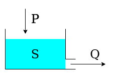
The single-element model is composed by a single reservoir governed by the differential equation

\[\frac{\textrm{d}S}{\textrm{d}t}=P-Q\]

where \(S\) is the state (storage) of the reservoir, \(P\) is the precipitation input, and \(Q\) is the outflow.

The outflow is defined by the equation:

\[Q = kS^\alpha\]

where \(k\) and \(\alpha\) are parameters of the element.

For simplicity, evapotranspiration is not considered in this demo.

The first step is to initialize the numerical approximator (see Numerical implementation). In this case, we will use the native Python implementation (i.e. not Numba) of the implicit Euler algorithm (numerical approximator) and the Pegasus algorithm (root finder). The initialization can be done with the following code, where the default settings of the solver are used (refer to the solver docstring).

solver_python = PegasusPython()

approximator = ImplicitEulerPython(root_finder=solver_python)

Note that the object approximator does not have internal states. Therefore, the same instance can be assigned to multiple elements.

The element is initialized next

reservoir = PowerReservoir(
    parameters={'k': 0.01, 'alpha': 2.0},
    states={'S0': 10.0},
    approximation=approximator,
    id='R'
)

During initialization, the two parameters (line 2) and the single initial state (line 3) are defined, together with the numerical approximator and the identifier. The identifier must be unique and cannot contain the character _, see Component identifiers.

After initialization, we specify the time step used to solve the differential equation and the inputs of the element.

reservoir.set_timestep(1.0)
reservoir.set_input([precipitation])

Here, precipitation is a Numpy array containing the precipitation time series. The length of the simulation (i.e., the number of time steps to run the model) is automatically set to the length of the input arrays.

The element can now be run

output = reservoir.get_output()[0]

The method get_output will run the element for all the time steps (solving the differential equation) and return a list containing all output arrays of the element. In this specific case there is only one output array, namely., the flow time series \(Q\).

The state of the reservoir at all time steps is saved in the attribute state_array of the element and can be accessed as follows

reservoir_state = reservoir.state_array[:, 0]

Here, state_array is a 2D array with the number of rows equal to the number of time steps, and the number of columns equal to the number of states. The order of states is defined in the docstring of the element.

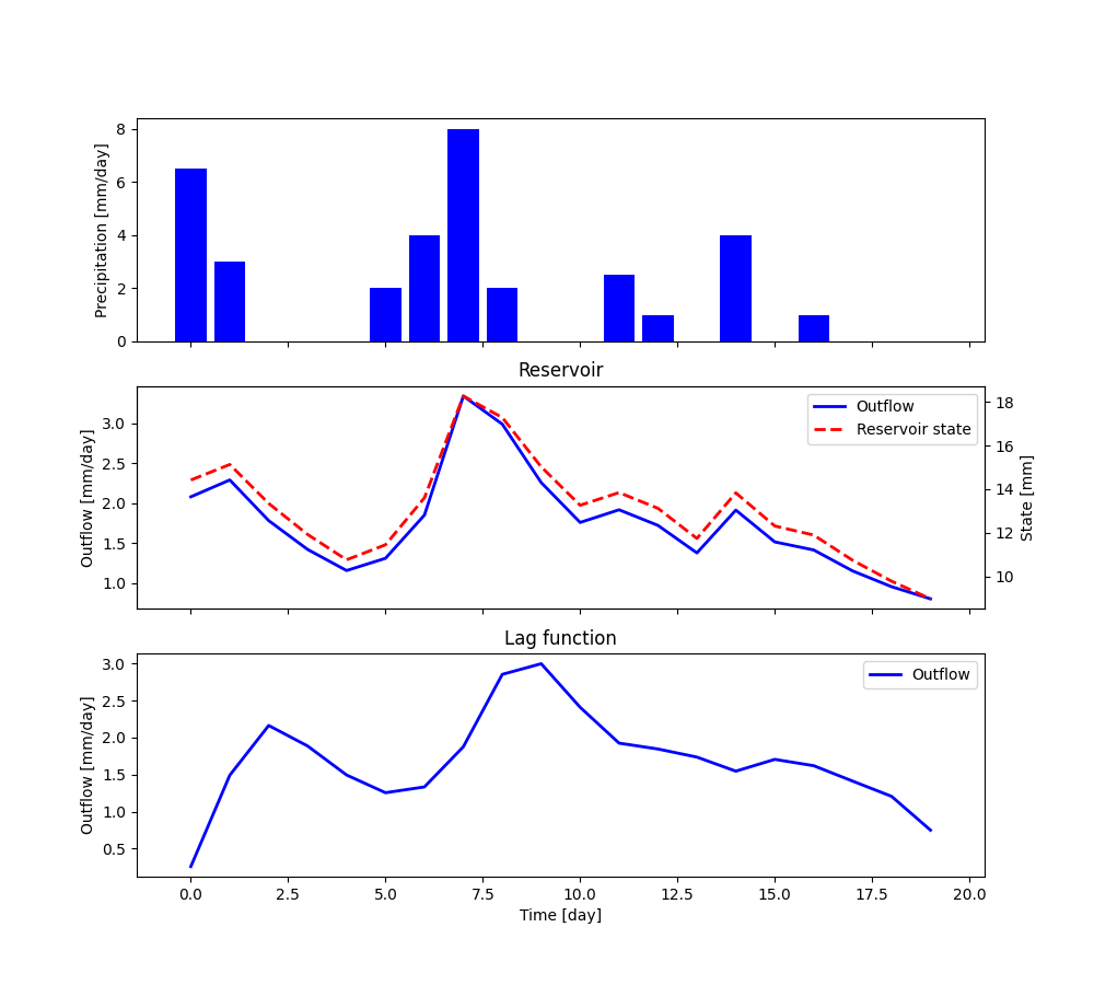
Finally, the simulation outputs can be plotted using standard Matplotlib functions, as follows

fig, ax = plt.subplots(2, 1, sharex=True, figsize=(10, 6))
ax[0].bar(x=range(len(precipitation)), height=precipitation, color='blue')
ax[1].plot(range(len(precipitation)), output, color='blue', lw=2, label='Outflow')
ax_bis = ax[1].twinx()
ax_bis.plot(range(len(precipitation)), reservoir_state, color='red', lw=2, ls='--', label='Reservoir state')

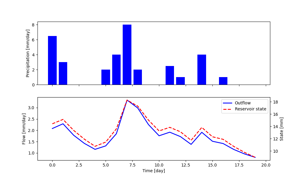
Note that the method get_output also sets the element states to their value at the final time step (in this case 8.98). As a consequence, if the method is called again, it will use this value as initial state instead of the one defined at initialization. This enables the modeler to continue the simulation at a later time, which can be useful in applications where new inputs arrive in real time. The states of the model can be reset using the method reset_states.

reservoir.reset_states()

Lumped model structure with 2 elements

We now move to a more complex model structure, where multiple elements are connected in a unit. For simplicity, we limit the complexity to two elements; more complex configurations can be found in the Application: implementation of existing conceptual models page.

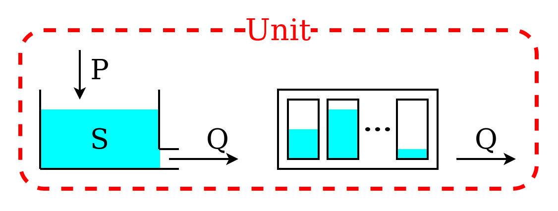
The unit structure comprises a reservoir that feeds a lag function. The lag function applies a convolution operation on the incoming fluxes

\[Q_{\textrm{out}}(t)= \int_{0}^{t} Q_{\textrm{in}}(t-\tau)h(\tau, t_{\textrm{lag}})\textrm{d}\tau\]

The behavior of the lag function is controlled by parameter \(t_{\textrm{lag}}\).

First, we initialize the two elements that compose the unit structure

reservoir = PowerReservoir(
    parameters={'k': 0.01, 'alpha': 2.0},
    states={'S0': 10.0},
    approximation=approximator,
    id='R'
)

lag_function = UnitHydrograph1(
    parameters={'lag-time': 2.3},
    states={'lag': None},
    id='lag-fun'
)

Note that the initial state of the lag function is set to None (line 10). The element will then initialize the state to an arrays of zeros of appropriate length, depending on the value of \(t_{\textrm{lag}}\); in this specific case, ceil(2.3) = 3.

Next, we initialize the unit that combines the elements

unit_1 = Unit(
    layers=[[reservoir], [lag_function]],
    id='unit-1'
)

Line 2 defines the unit structure: it is a 2D list where the inner level sets the elements belonging to each layer and the outer level lists the layers.

After initialization, time step size and inputs are defined

unit_1.set_timestep(1.0)
unit_1.set_input([precipitation])

The unit sets the time step size for all its elements and transfers the inputs to the first element (in this example, to the reservoir).

The unit can now be run

output = unit_1.get_output()[0]

In this code, the unit will call the get_output method of all its elements (from upstream to downstream), set the inputs of the downstream elements to the output of their respective upstream elements, and return the output of the last element.

After the unit simulation has completed, the outputs and the states of its elements can be retrieved as follows

r_state = unit_1.get_internal(id='R', attribute='state_array')[:, 0]
r_output = unit_1.call_internal(id='R', method='get_output', solve=False)[0]

Note that in line 2 we pass the argument solve=False to the function get_output, in order to access the computed states and outputs without re-running the reservoir element.

The plot shows the output of the simulation (obtained by plotting output, r_state, and r_output).

If we wish to re-run the model, the elements of the unit can be re-set to their initial state

unit_1.reset_states()

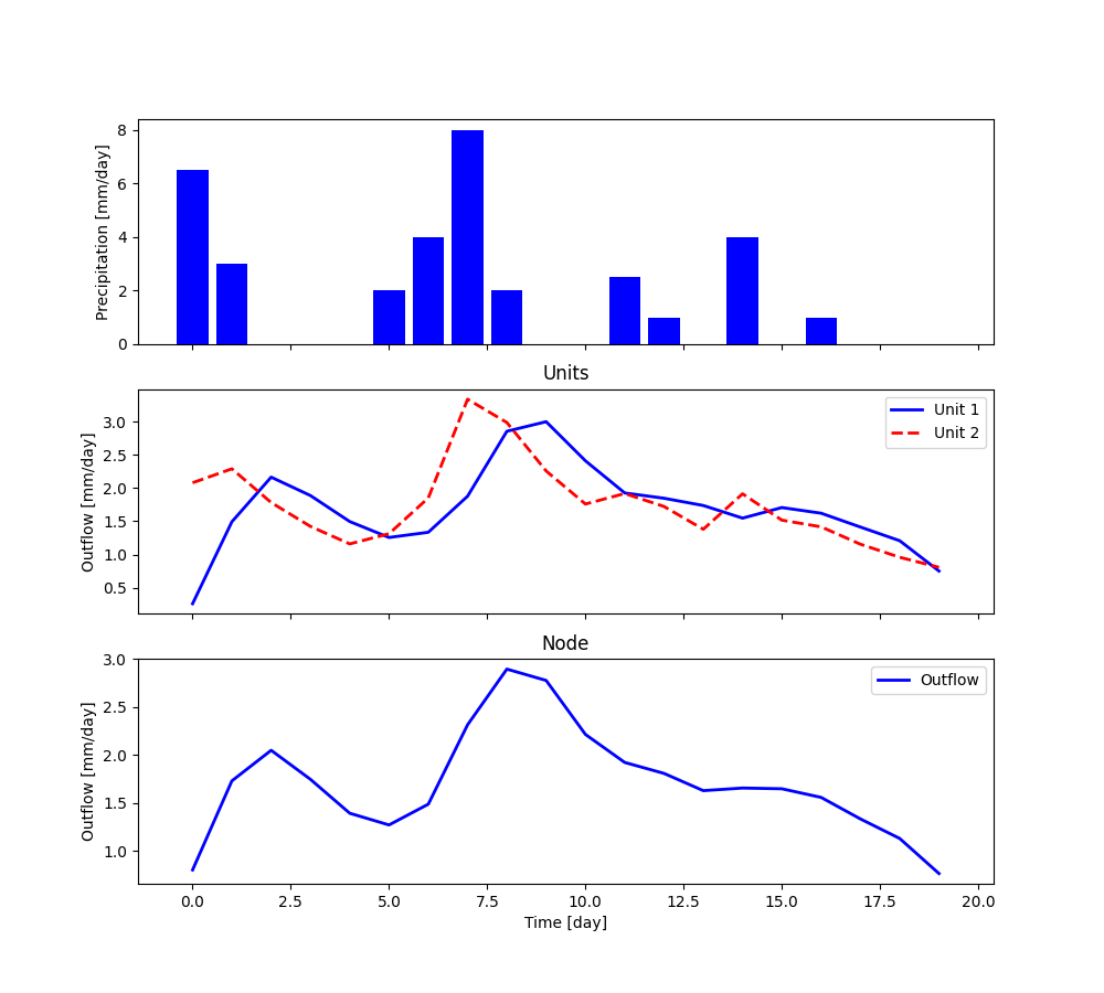
Simple semi-distributed model

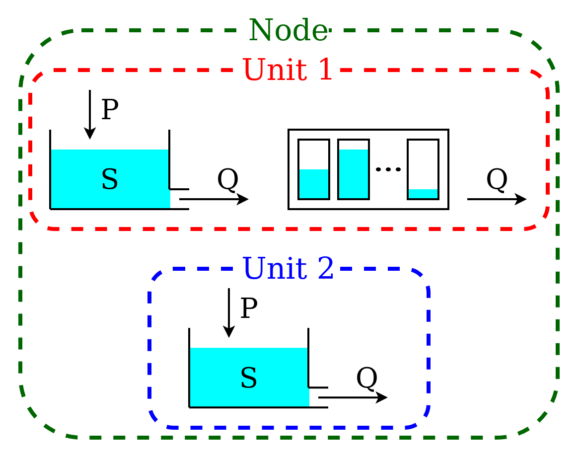
This model is intended to represent a spatially semi-distributed configuration. A node is used to represent a catchment with multiple areas that react differently to the same inputs. In this example, we represent 70% of the catchment using the structure described in Lumped model structure with 2 elements, and the remaining 30% using a single reservoir.

This model configuration is achieved using a node with multiple units.

First, we initialize the two units and the elements composing them, in the same way as in the previous sections.

reservoir = PowerReservoir(
    parameters={'k': 0.01, 'alpha': 2.0},
    states={'S0': 10.0},
    approximation=approximator,
    id='R'
)

lag_function = UnitHydrograph1(
    parameters={'lag-time': 2.3},
    states={'lag': None},
    id='lag-fun'
)

unit_1 = Unit(
    layers=[[reservoir], [lag_function]],
    id='unit-1'
)

unit_2 = Unit(
    layers=[[reservoir]],
    id='unit-2'
)

Note that, once the elements are added to a unit, they become independent, meaning that any change to the reservoir contained in unit_1 does not affect the reservoir contained in unit_2 (see Unit).

The next step is to initialize the node, which combines the two units

node_1 = Node(
    units=[unit_1, unit_2],
    weights=[0.7, 0.3],
    area=10.0,
    id='node-1'
)

Line 2 contains the list of units that belong to the node, and line 3 gives their weight (i.e. the portion of the node outflow coming from each unit). Line 4 specifies the representative area of the node.

Next, we define the time step size and the model inputs

node_1.set_timestep(1.0)
node_1.set_input([precipitation])

The same time step size will be assigned to all elements within the node, and the inputs will be passed to all the units of the node.

We can now run the node and collect its output

output = node_1.get_output()[0]

The node will call the method get_output of all its units and aggregate their outputs using the weights.

The outputs of the single units, as well as the states and fluxes of the elements composing them, can be retrieved using the method call_internal

output_unit_1 = node_1.call_internal(id='unit-1', method='get_output', solve=False)[0]
output_unit_2 = node_1.call_internal(id='unit-2', method='get_output', solve=False)[0]

The plot shows the output of the simulation.

All elements within the node can be re-set to their initial states

node_1.reset_states()

Semi-distributed model with multiple nodes

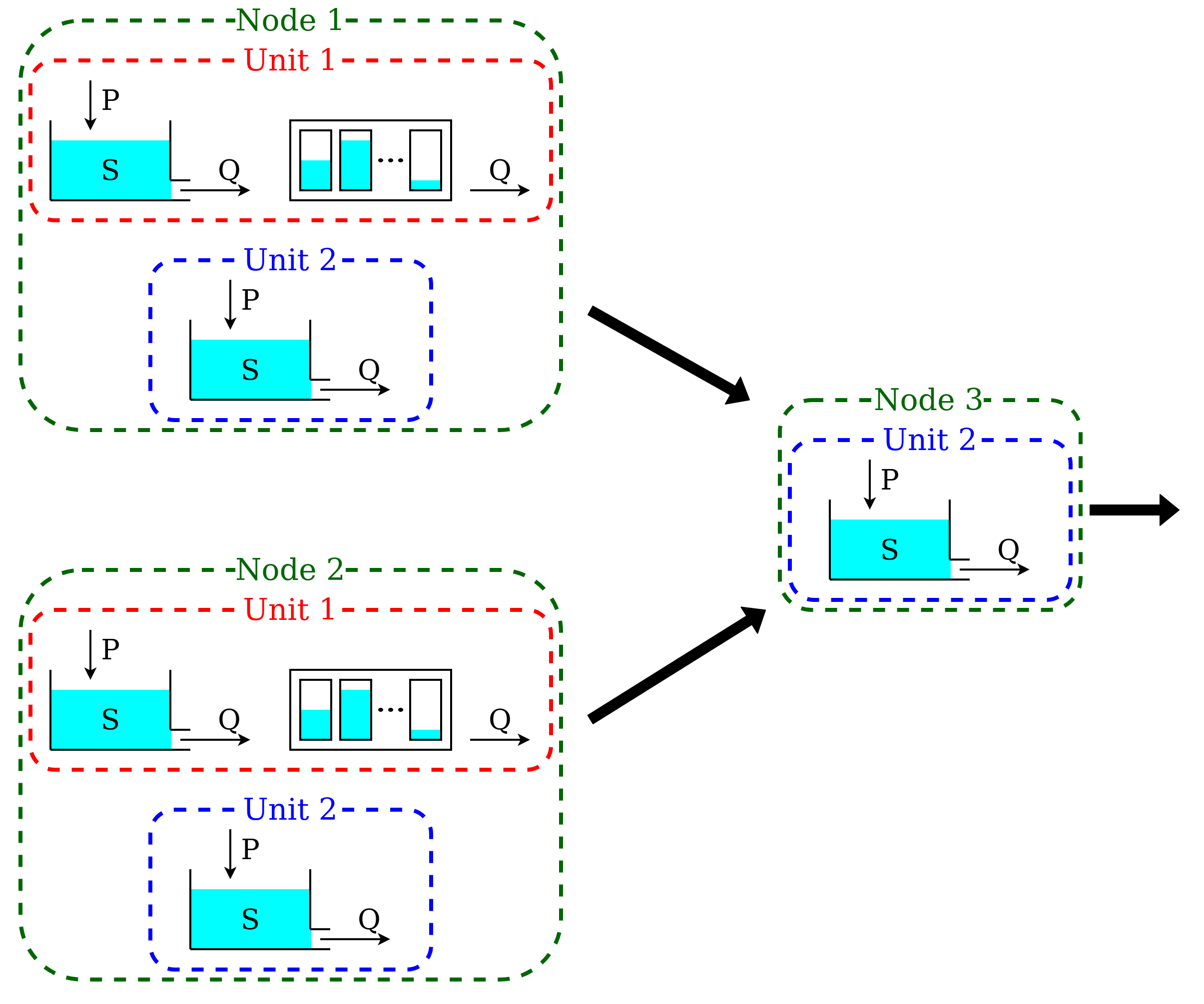
A catchment can be composed by several subcatchments (nodes) connected in a network. Each subcatchment receives its own inputs, but may share parameter values with other subcatchments with the same units.

This semi-distributed configuration can be implemented in SuperflexPy by creating a network with multiple nodes.

First, we initialize the nodes

reservoir = PowerReservoir(
    parameters={'k': 0.01, 'alpha': 2.0},
    states={'S0': 10.0},
    approximation=approximator,
    id='R'
)

lag_function = UnitHydrograph1(
    parameters={'lag-time': 2.3},
    states={'lag': None},
    id='lag-fun'
)

unit_1 = Unit(
    layers=[[reservoir], [lag_function]],
    id='unit-1'
)

unit_2 = Unit(
    layers=[[reservoir]],
    id='unit-2'
)

node_1 = Node(
    units=[unit_1, unit_2],
    weights=[0.7, 0.3],
    area=10.0,
    id='node-1'
)

node_2 = Node(
    units=[unit_1, unit_2],
    weights=[0.3, 0.7],
    area=5.0,
    id='node-2'
)

node_3 = Node(
    units=[unit_2],
    weights=[1.0],
    area=3.0,
    id='node-3'
)

Here, nodes node_1 and node_2 contain both units, unit_1 and unit_2, but in different proportions. Node node_3 contains only a single unit, unit_2.

When units are added to a node, the states of the elements within the units remain independent while the parameters stay linked. In this example the change of a parameter in unit_1 in node_1 is applied also to unit_1 in node_2. This “shared parameters” behavior can be disabled by setting the parameter shared_parameters to False when initializing the nodes (see Node)

The network is initialized as follows

net = Network(
    nodes=[node_1, node_2, node_3],
    topology={
        'node-1': 'node-3',
        'node-2': 'node-3',
        'node-3': None
    }
)

Line 2 provides the list of the nodes belonging to the network. Lines 4-6 define the connectivity of the network; this is done using a dictionary with the keys given by the node identifiers and values given by the single downstream node. The most downstream node has, by convention, its value set to None.

The inputs are catchment-specific and must be provided to each node.

node_1.set_input([precipitation])
node_2.set_input([precipitation * 0.5])
node_3.set_input([precipitation + 1.0])

The time step size is defined at the network level.

net.set_timestep(1.0)

We can now run the network and get the output values

output = net.get_output()

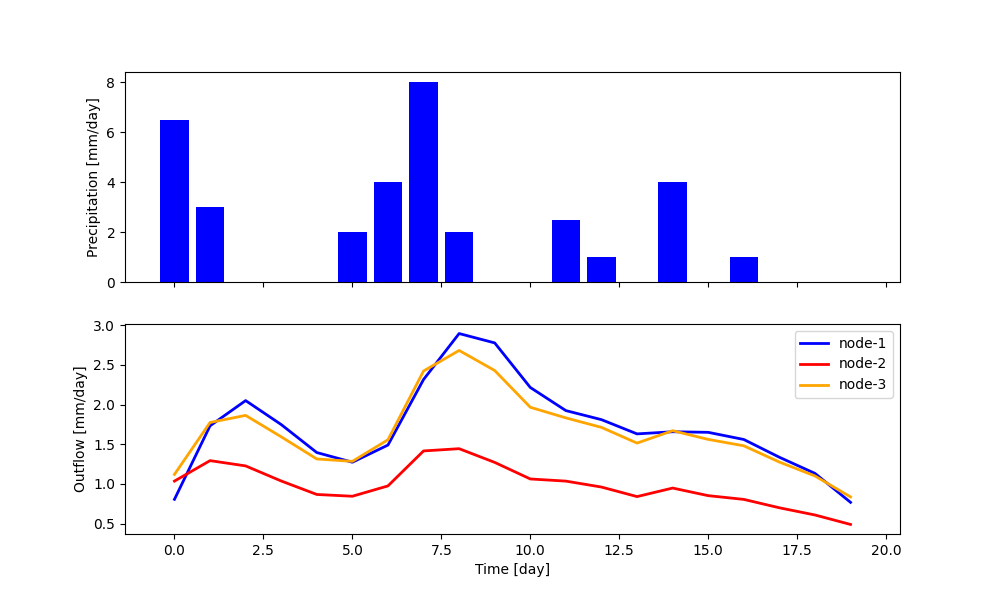
The network runs the nodes from upstream to downstream, collects their outputs, and routes them to the outlet. The output of the network is a dictionary, with keys given by the node identifiers and values given by the list of output fluxes of the nodes. It is also possible to retrieve the internals (e.g. fluxes, states, etc.) of the nodes.

output_unit_1_node_1 = net.call_internal(id='node-1_unit-1',
                                         method='get_output',
                                         solve=False)[0]

The plot shows the results of the simulation.