Case studies

This page describes the model configurations used in research publications based on Superflex and SuperflexPy.

Dal Molin et al., 2020, HESS

This section describes the implementation of the semi-distributed hydrological model M02 presented in the article:

Dal Molin, M., Schirmer, M., Zappa, M., and Fenicia, F.: Understanding dominant controls on streamflow spatial variability to set up a semi-distributed hydrological model: the case study of the Thur catchment, Hydrol. Earth Syst. Sci., 24, 1319–1345, https://doi.org/10.5194/hess-24-1319-2020, 2020.

In this application, the Thur catchment is discretized into 10 subcatchments and 2 hydrological response units (HRUs). Please refer to the article for the details; here we only show the SuperflexPy code needed to reproduce the model from the publication.

Model structure

The two HRUs are represented using the same model structure, shown in the figure below.

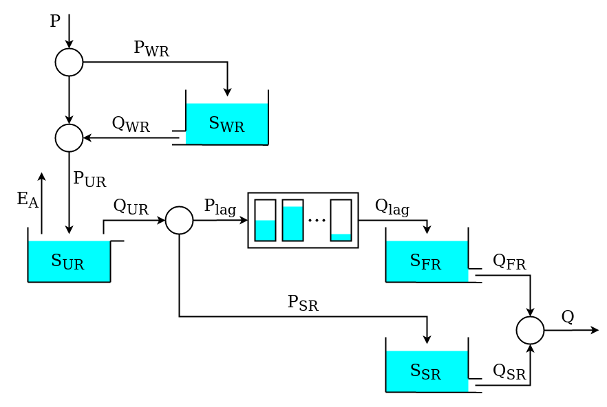
This model structure is similar to HYMOD; its implementation using SuperflexPy is presented next.

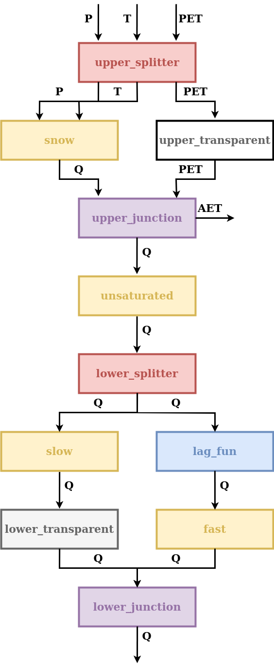
This model structure includes a snow model, and hence requires time series of temperature as an input in addition to precipitation and PET. Inputs are assigned to the element in the first layer of the unit and the model structure then propagates these inputs through all the elements until they reach the element (snow reservoir) where they are actually needed. Consequently, all the elements upstream of the snow reservoir have to be able to handle (i.e. to input and output) that input.

In this model, the choice of temperature as input is convenient because temperature is required by the element appearing first in the model structure.

In other cases, an alternative solution would have been to design the snow reservoir such that the temperature is one of its state variables. This solution would be preferable if the snow reservoir is not the first element of the structure, given that temperature is not an input commonly used by other elements.

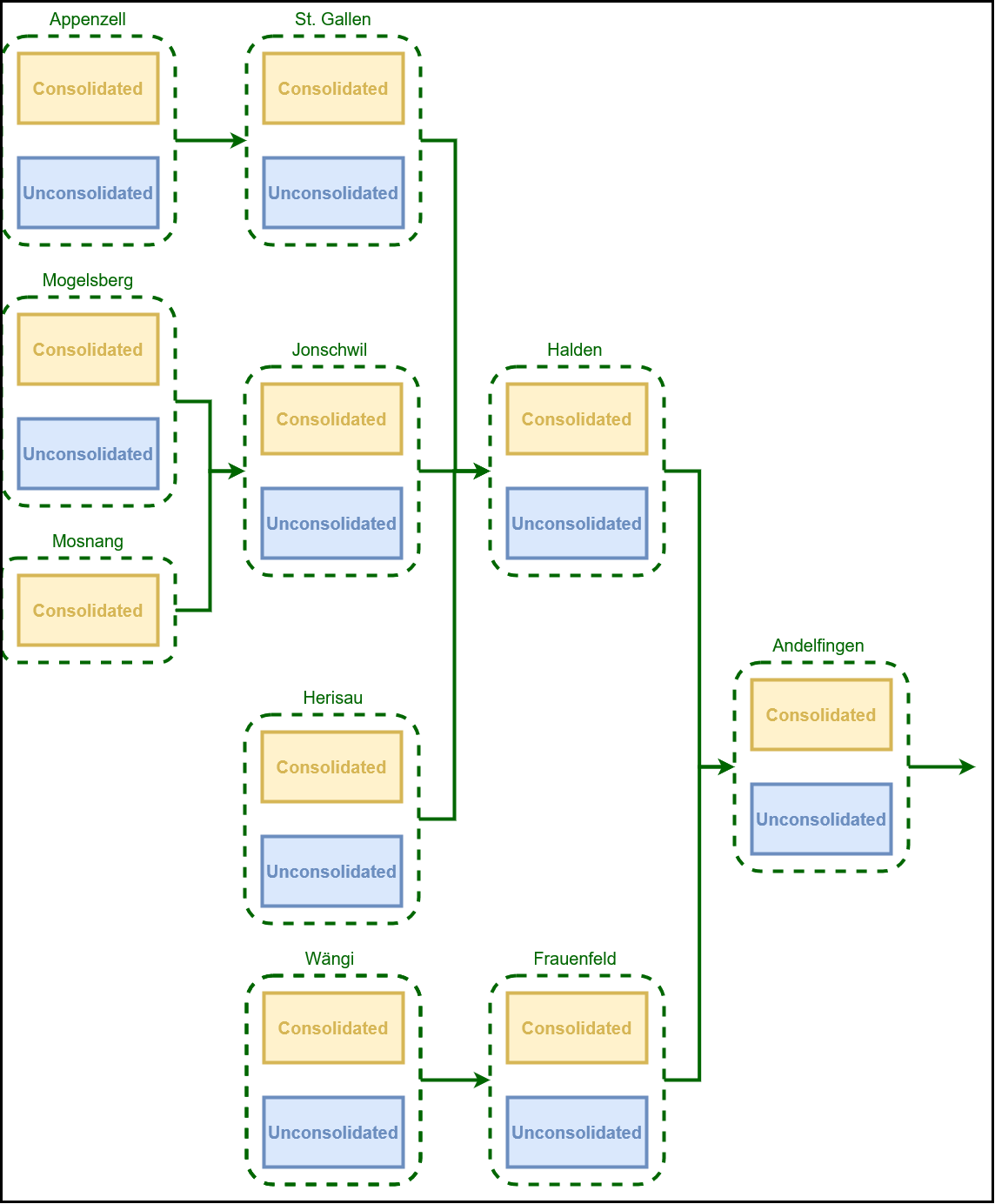
The discretization of the Thur catchment into units (HRUs) and nodes (subcatchments) is represented in the figure below.

Initializing the elements

All elements required for this model structure are already available in SuperflexPy. Therefore they just need to be imported.

from superflexpy.implementation.elements.thur_model_hess import SnowReservoir, UnsaturatedReservoir, HalfTriangularLag, PowerReservoir
from superflexpy.implementation.elements.structure_elements import Transparent, Junction, Splitter
from superflexpy.implementation.root_finders.pegasus import PegasusPython
from superflexpy.implementation.numerical_approximators.implicit_euler import ImplicitEulerPython

Elements are then initialized, defining the initial state and parameter values.

solver = PegasusPython()
approximator = ImplicitEulerPython(root_finder=solver)

upper_splitter = Splitter(
    direction=[
        [0, 1, None],    # P and T go to the snow reservoir
        [2, None, None]  # PET goes to the transparent element
    ],
    weight=[
        [1.0, 1.0, 0.0],
        [0.0, 0.0, 1.0]
    ],
    id='upper-splitter'
)

snow = SnowReservoir(
    parameters={'t0': 0.0, 'k': 0.01, 'm': 2.0},
    states={'S0': 0.0},
    approximation=approximator,
    id='snow'
)

upper_transparent = Transparent(
    id='upper-transparent'
)

upper_junction = Junction(
    direction=[
        [0, None],
        [None, 0]
    ],
    id='upper-junction'
)

unsaturated = UnsaturatedReservoir(
    parameters={'Smax': 50.0, 'Ce': 1.0, 'm': 0.01, 'beta': 2.0},
    states={'S0': 10.0},
    approximation=approximator,
    id='unsaturated'
)

lower_splitter = Splitter(
    direction=[
        [0],
        [0]
    ],
    weight=[
        [0.3],   # Portion to slow reservoir
        [0.7]    # Portion to fast reservoir
    ],
    id='lower-splitter'
)

lag_fun = HalfTriangularLag(
    parameters={'lag-time': 2.0},
    states={'lag': None},
    id='lag-fun'
)

fast = PowerReservoir(
    parameters={'k': 0.01, 'alpha': 3.0},
    states={'S0': 0.0},
    approximation=approximator,
    id='fast'
)

slow = PowerReservoir(
    parameters={'k': 1e-4, 'alpha': 1.0},
    states={'S0': 0.0},
    approximation=approximator,
    id='slow'
)

lower_transparent = Transparent(
    id='lower-transparent'
)

lower_junction = Junction(
    direction=[
        [0, 0]
    ],
    id='lower-junction'
)

Initializing the HRUs structure

We now define the two units that represent the HRUs.

consolidated = Unit(
    layers=[
        [upper_splitter],
        [snow, upper_transparent],
        [upper_junction],
        [unsaturated],
        [lower_splitter],
        [slow, lag_fun],
        [lower_transparent, fast],
        [lower_junction],
    ],
    id='consolidated'
)

unconsolidated = Unit(
    layers=[
        [upper_splitter],
        [snow, upper_transparent],
        [upper_junction],
        [unsaturated],
        [lower_splitter],
        [slow, lag_fun],
        [lower_transparent, fast],
        [lower_junction],
    ],
    id='unconsolidated'
)

Initializing the catchments

We now assign the units (HRUs) to the nodes (catchments).

andelfingen = Node(
    units=[consolidated, unconsolidated],
    weights=[0.24, 0.76],
    area=403.3,
    id='andelfingen'
)

appenzell = Node(
    units=[consolidated, unconsolidated],
    weights=[0.92, 0.08],
    area=74.4,
    id='appenzell'
)

frauenfeld = Node(
    units=[consolidated, unconsolidated],
    weights=[0.49, 0.51],
    area=134.4,
    id='frauenfeld'
)

halden = Node(
    units=[consolidated, unconsolidated],
    weights=[0.34, 0.66],
    area=314.3,
    id='halden'
)

herisau = Node(
    units=[consolidated, unconsolidated],
    weights=[0.88, 0.12],
    area=16.7,
    id='herisau'
)

jonschwil = Node(
    units=[consolidated, unconsolidated],
    weights=[0.9, 0.1],
    area=401.6,
    id='jonschwil'
)

mogelsberg = Node(
    units=[consolidated, unconsolidated],
    weights=[0.92, 0.08],
    area=88.1,
    id='mogelsberg'
)

mosnang = Node(
    units=[consolidated],
    weights=[1.0],
    area=3.1,
    id='mosnang'
)

stgallen = Node(
    units=[consolidated, unconsolidated],
    weights=[0.87, 0.13],
    area=186.6,
    id='stgallen'
)

waengi = Node(
    units=[consolidated, unconsolidated],
    weights=[0.63, 0.37],
    area=78.9,
    id='waengi'
)

Note that all nodes incorporate the information about their area, which is used by the network to calculate their contribution to the total outflow.

There is no requirement for a node to contain all units. For example, the unit unconsolidated is not present in the Mosnang subcatchment. Hence, as shown in line 50, the node mosnang is defined to contain only the unit consolidated.

Initializing the network

The last step consists in creating the network that connects all the nodes previously initialized.

thur_catchment = Network(
    nodes=[
        andelfingen,
        appenzell,
        frauenfeld,
        halden,
        herisau,
        jonschwil,
        mogelsberg,
        mosnang,
        stgallen,
        waengi,
    ],
    topology={
        'andelfingen': None,
        'appenzell': 'stgallen',
        'frauenfeld': 'andelfingen',
        'halden': 'andelfingen',
        'herisau': 'halden',
        'jonschwil': 'halden',
        'mogelsberg': 'jonschwil',
        'mosnang': 'jonschwil',
        'stgallen': 'halden',
        'waengi': 'frauenfeld',
    }
)

Running the model

Before the model can be run, we need to set the input fluxes and the time step size.

The input fluxes are assigned to the individual nodes (catchments). Here, the data is available as a Pandas DataFrame, with columns names P_name_of_the_catchment, T_name_of_the_catchment, and PET_name_of_the_catchment.

The inputs can be set using a for loop

for cat, cat_name in zip(catchments, catchments_names):
    cat.set_input([
        df['P_{}'.format(cat_name)].values,
        df['T_{}'.format(cat_name)].values,
        df['PET_{}'.format(cat_name)].values,
    ])

The model time step size is set next. This can be done directly at the network level, which automatically sets the time step size to all lower-level model components.

thur_catchment.set_timestep(1.0)

We can now run the model and access its output (see Semi-distributed model with multiple nodes for details).

output = thur_catchment.get_output()