Note

Last update 04/05/2021

List of currently implemented elements

SuperflexPy provides four levels of components (elements, units, nodes and network) for constructing conceptual hydrological models. The components presented in the page Organization of SuperflexPy represent the core of SuperflexPy. These components can be extended to create customized models.

Most of the customization efforts will be required for elements (i.e., reservoirs, lag, and connection elements). This page describes all elements that have been created and shared by the community of SuperflexPy. These elements can be used to construct a wide range of model structures.

This section lists elements according to their type, namely

Reservoir
Lag elements
Connections

Within each section, the elements are listed in alphabetical order.

Reservoirs

Interception filter

This reservoir is used to simulate interception in models, including GR4J. Further details are provided in the page GR4J.

from superflexpy.implementation.elements.gr4j import InterceptionFilter

Inputs

Potential evapotranspiration \(E^{\textrm{in}}_{\textrm{POT}}\ [LT^{-1}]\)
Precipitation \(P^{\textrm{in}}\ [LT^{-1}]\)

Outputs from `get_output`

Net potential evapotranspiration \(E^{\textrm{out}}_{\textrm{POT}}\ [LT^{-1}]\)
Net precipitation \(P^{\textrm{out}}\ [LT^{-1}]\)

Governing equations

\[\begin{split}& \textrm{if } P^{\textrm{in}} > E^{\textrm{in}}_{\textrm{POT}}: \\ & \quad P^{\textrm{out}} = P^{\textrm{in}} - E^{\textrm{in}}_{\textrm{POT}} \\ & \quad E^{\textrm{out}}_{\textrm{POT}} = 0 \\ \\ & \textrm{if } P^{\textrm{in}} < E^{\textrm{in}}_{\textrm{POT}}: \\ & \quad P^{\textrm{out}} = 0 \\ & \quad E^{\textrm{out}}_{\textrm{POT}} = E^{\textrm{in}}_{\textrm{POT}} - P^{\textrm{in}}\end{split}\]

Linear reservoir

This reservoir assumes a linear storage-discharge relationship. It represents arguably the simplest hydrological model. For example, it is used in the model HYMOD to simulate channel routing and lower-zone storage processes. Further details are provided in the page HYMOD.

from superflexpy.implementation.elements.hymod import LinearReservoir

Inputs

Precipitation \(P\ [LT^{-1}]\)

Outputs from `get_output`

Total outflow \(Q\ [LT^{-1}]\)

Governing equations

\[\begin{split}& \frac{\textrm{d}S}{\textrm{d}{t}}=P - Q \\ & Q=kS\end{split}\]

Power reservoir

This reservoir assumes that the storage-discharge relationship is described by a power function. This type of reservoir is common in hydrological models. For example, it is used in the HBV family of models to represent the fast response of a catchment.

from superflexpy.implementation.elements.hbv import PowerReservoir

Inputs

Precipitation \(P\ [LT^{-1}]\)

Outputs from `get_output`

Total outflow \(Q\ [LT^{-1}]\)

Governing equations

\[\begin{split}& \frac{\textrm{d}S}{\textrm{d}{t}}=P - Q \\ & Q=kS^{\alpha}\end{split}\]

Production store (GR4J)

This reservoir is used to simulate runoff generation in the model GR4J. Further details are provided in the page GR4J.

from superflexpy.implementation.elements.gr4j import ProductionStore

Inputs

Potential evapotranspiration \(E_{\textrm{pot}}\ [LT^{-1}]\)
Precipitation \(P\ [LT^{-1}]\)

Outputs from `get_output`

Total outflow \(P_{\textrm{r}}\ [LT^{-1}]\)

Secondary outputs

Actual evapotranspiration \(E_{\textrm{act}}\ [LT^{-1}]\) get_aet()

Governing equations

\[\begin{split}& \frac{\textrm{d}S}{\textrm{d}{t}}=P_{\textrm{s}}-E_{\textrm{act}}-Q_{\textrm{perc}} \\ & P_{\textrm{s}}=P\left(1-\left(\frac{S}{x_1}\right)^\alpha\right) \\ & E_{\textrm{act}}=E_{\textrm{pot}}\left(2\frac{S}{x_1}-\left(\frac{S}{x_1}\right)^\alpha\right) \\ & Q_{\textrm{perc}} = \frac{{x_1}^{1-\beta}}{(\beta-1)}\nu^{\beta-1}S^{\beta} \\ & P_{\textrm{r}}=P - P_{\textrm{s}} + Q_{\textrm{perc}}\end{split}\]

Routing store (GR4J)

This reservoir is used to simulate routing in the model GR4J. Further details are provided in the page GR4J.

from superflexpy.implementation.elements.gr4j import RoutingStore

Inputs

Precipitation \(P\ [LT^{-1}]\)

Outputs from `get_output`

Outflow \(Q\ [LT^{-1}]\)
Loss term \(F\ [LT^{-1}]\)

Governing equations

\[\begin{split}& \frac{\textrm{d}S}{\textrm{d}{t}}=P-Q-F \\ & Q=\frac{x_3^{1-\gamma}}{(\gamma-1)}S^{\gamma} \\ & F = \frac{x_2}{x_3^{\omega}}S^{\omega}\end{split}\]

Snow reservoir

This reservoir is used to simulate snow processes based on temperature. Further details are provided in the section Dal Molin et al., 2020, HESS.

from superflexpy.implementation.elements.thur_model_hess import SnowReservoir

Inputs

Precipitation \(P\ [LT^{-1}]\)
Temperature \(T\ [°C]\)

Outputs from `get_output`

Sum of snow melt and rainfall input \(=P-P_{\textrm{snow}}+M\ [LT^{-1}]\)

Governing equations

\[\begin{split}& \frac{\textrm{d}S}{\textrm{d}{t}}=P_{\textrm{snow}}-M \\ & P_{\textrm{snow}}=P\quad\textrm{if } T\leq T_0;\quad\textrm{else } 0 \\ & M = M_{\textrm{pot}}\left(1-\exp\left(-\frac{S}{m}\right)\right) \\ & M_{\textrm{pot}}=kT\quad\textrm{if } T\geq T_0;\quad\textrm{else } 0 \\\end{split}\]

Unsaturated reservoir (inspired to HBV)

This reservoir specifies the actual evapotranspiration as a smoothed threshold function of storage, in combination with the storage-discharge relationship being set to a power function. It is inspired by the HBV family of models, where a similar approach (but without smoothing) is used to represent unsaturated soil dynamics.

from superflexpy.implementation.elements.hbv import UnsaturatedReservoir

Inputs

Precipitation \(P\ [LT^{-1}]\)
Potential evapotranspiration \(E_{\textrm{pot}}\ [LT^{-1}]\)

Outputs from `get_output`

Total outflow \(Q\ [LT^{-1}]\)

Secondary outputs

Actual evapotranspiration \(E_{\textrm{act}}\) get_AET()

Governing equations

\[\begin{split}& \frac{\textrm{d}S}{\textrm{d}{t}}=P - E_{\textrm{act}} - Q \\ & \overline{S} = \frac{S}{S_{\textrm{max}}} \\ & E_{\textrm{act}}=C_{\textrm{e}}E_{\textrm{pot}}\left(\frac{\overline{S}(1+m)}{\overline{S}+m}\right) \\ & Q=P\left(\overline{S}\right)^{\beta}\end{split}\]

Upper zone (HYMOD)

This reservoir is part of the HYMOD model and is used to simulate the upper soil zone. Further details are provided in the page HYMOD.

from superflexpy.implementation.elements.hymod import UpperZone

Inputs

Precipitation \(P\ [LT^{-1}]\)
Potential evapotranspiration \(E_{\textrm{pot}}\ [LT^{-1}]\)

Outputs from `get_output`

Total outflow \(Q\ [LT^{-1}]\)

Secondary outputs

Actual evapotranspiration \(E_{\textrm{act}}\ [LT^{-1}]\) get_AET()

Governing equations

\[\begin{split}& \frac{\textrm{d}S}{\textrm{d}{t}}=P - E_{\textrm{act}} - Q \\ & \overline{S} = \frac{S}{S_{\textrm{max}}} \\ & E_{\textrm{act}}=E_{\textrm{pot}}\left(\frac{\overline{S}(1+m)}{\overline{S}+m}\right) \\ & Q=P\left(1-\left(1-\overline{S}\right)^{\beta}\right)\end{split}\]

Lag elements

All lag elements implemented in SuperflexPy can accommodate an arbitrary number of input fluxes, and apply a convolution based on a weight array that defines the shape of the lag function.

Lag elements differ solely in the definition of the weight array. The nature (i.e., number and order) of inputs and outputs depend on the element upstream of the lag element.

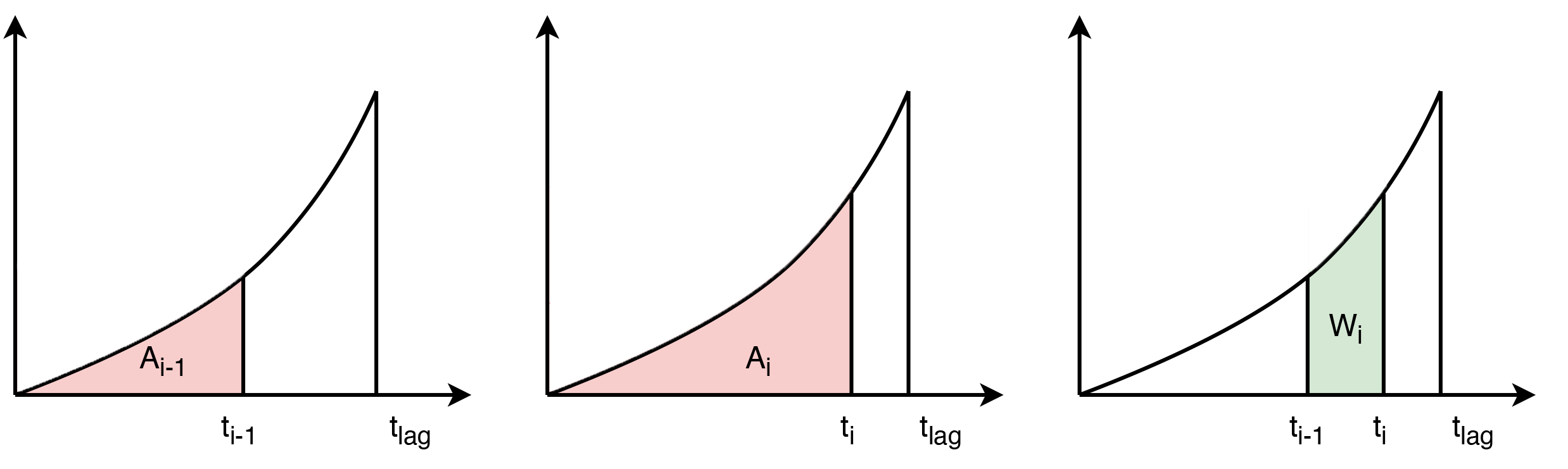
The weight array can be defined by giving the area below the lag function as a function of the time coordinate. The maximum lag \(t_{\textrm{lag}}\) must also be specified. The weights are then given by differences between the values of the area at consecutive lags. This approach is shown in the figure above, where the weight \(W_i\) is calculated as the difference between areas \(A_i\) and \(A_{i-1}\).

Half triangular lag

This lag element implements the element present in the case study Dal Molin et al., 2020, HESS and used in other Superflex studies.

from superflexpy.implementation.elements.thur_model_hess import HalfTriangularLag

Definition of weight array

The area below the lag function is given by

\[\begin{split}&A_{\textrm{lag}}(t) = 0 & \quad \textrm{for } t \leq 0\\ &A_{\textrm{lag}}(t) = \left(\frac{t}{t_{\textrm{lag}}}\right)^2 & \quad \textrm{for } 0< t \leq t_{\textrm{lag}}\\ &A_{\textrm{lag}}(t) = 1 & \quad \textrm{for } t > t_{\textrm{lag}}\end{split}\]

The weight array is then calculated as

\[w(t_{\textrm{i}}) = A_{\textrm{lag}}(t_{\textrm{i}}) - A_{\textrm{lag}}(t_{\textrm{i-1}})\]

Unit hydrograph 1 (GR4J)

This lag element implements the unit hydrograph 1 of GR4J.

from superflexpy.implementation.elements.gr4j import UnitHydrograph1

Definition of weight array

The area below the lag function is given by

\[\begin{split}&A_{\textrm{lag}}(t) = 0 & \quad \textrm{for } t \leq 0\\ &A_{\textrm{lag}}(t) = \left(\frac{t}{t_{\textrm{lag}}}\right)^\frac{5}{2} & \quad \textrm{for } 0< t \leq t_{\textrm{lag}}\\ &A_{\textrm{lag}}(t) = 1 & \quad \textrm{for } t > t_{\textrm{lag}}\end{split}\]

The weight array is then calculated as

\[w(t_{\textrm{i}}) = A_{\textrm{lag}}(t_{\textrm{i}}) - A_{\textrm{lag}}(t_{\textrm{i-1}})\]

Unit hydrograph 2 (GR4J)

This lag element implements the unit hydrograph 2 of GR4J.

from superflexpy.implementation.elements.gr4j import UnitHydrograph2

Definition of weight array

The area below the lag function is given by

\[\begin{split}&A_{\textrm{lag}}(t) = 0 & \quad \textrm{for } t \leq 0\\ &A_{\textrm{lag}}(t) = \frac{1}{2}\left(\frac{2t}{t_{\textrm{lag}}}\right)^\frac{5}{2} & \quad \textrm{for } 0< t \leq \frac{t_{\textrm{lag}}}{2}\\ &A_{\textrm{lag}}(t) = 1 - \frac{1}{2}\left(2-\frac{2t}{t_{\textrm{lag}}}\right)^\frac{5}{2} & \quad \textrm{for } \frac{t_{\textrm{lag}}}{2}< t \leq t_{\textrm{lag}}\\ &A_{\textrm{lag}}(t) = 1 & \quad \textrm{for } t > t_{\textrm{lag}}\end{split}\]

The weight array is then calculated as

\[w(t_{\textrm{i}}) = A_{\textrm{lag}}(t_{\textrm{i}}) - A_{\textrm{lag}}(t_{\textrm{i-1}})\]

Connections

SuperflexPy implements four connection elements:

splitter
junction
linker
transparent element

In addition, customized connectors have been implemented to achieve specific model designs. These customized elements are listed in this section.

Flux aggregator (GR4J)

This element is used to combine routing, exchange and outflow fluxes in the GR4J model. Further details are provided in the page GR4J.

from superflexpy.implementation.elements.gr4j import FluxAggregator

Inputs

Outflow routing store \(Q_{\textrm{RR}}\ [LT^{-1}]\)
Exchange flux \(Q_{\textrm{RF}}\ [LT^{-1}]\)
Outflow UH2 \(Q_{\textrm{UH2}}\ [LT^{-1}]\)

Main outputs

Outflow \(Q\ [LT^{-1}]\)

Governing equations

\[\begin{split}& Q = Q_{\textrm{RR}} + \max(0;Q_{\textrm{UH2}} - Q_{\textrm{RF}}) \\\end{split}\]

List of currently implemented elements

Reservoirs

Interception filter

Inputs

Outputs from get_output

Governing equations

Linear reservoir

Inputs

Outputs from get_output

Governing equations

Power reservoir

Inputs

Outputs from get_output

Governing equations

Production store (GR4J)

Inputs

Outputs from get_output

Secondary outputs

Governing equations

Routing store (GR4J)

Inputs

Outputs from get_output

Governing equations

Snow reservoir

Inputs

Outputs from get_output

Governing equations

Unsaturated reservoir (inspired to HBV)

Inputs

Outputs from get_output

Secondary outputs

Governing equations

Upper zone (HYMOD)

Inputs

Outputs from get_output

Secondary outputs

Governing equations

Lag elements

Half triangular lag

Definition of weight array

Unit hydrograph 1 (GR4J)

Definition of weight array

Unit hydrograph 2 (GR4J)

Definition of weight array

Connections

Flux aggregator (GR4J)

Inputs

Main outputs

Governing equations

Outputs from `get_output`

Outputs from `get_output`

Outputs from `get_output`

Outputs from `get_output`

Outputs from `get_output`

Outputs from `get_output`

Outputs from `get_output`

Outputs from `get_output`