Note
Last update 21/07/2021
Note
If you build your own SuperflexPy element, we would appreciate if you share your implementation with the community (see Software organization and contribution). Please remember to update the List of currently implemented elements page to make other users aware of your implementation.
Expand SuperflexPy: Build customized elements
This page illustrates how to create customized elements using the SuperflexPy framework.
The examples include three elements:
Linear reservoir
Half-triangular lag function
Parameterized splitter
The customized elements presented here are relatively simple, in order to
provide a clear illustration of the programming approach. To gain a deeper
understanding of SuperflexPy functionalities, please familiarize with the code of
existing elements (importing “path” superflexpy.implementation.elements).
Linear reservoir
This section presents the implementation of a linear reservoir element from
the generic class ODEsElement.
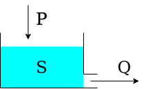
The reservoir is controlled by the following differential equation
with
Note that the differential equation can be solved analytically, and (if applied) the implicit Euler numerical approximation does not require iteration. However, we will still use the numerical approximator offered by SuperflexPy (see Numerical implementation) to illustrate how to proceed in a more general case where analytical solutions are not available.
The SuperflexPy framework provides the class ODEsElement, which has most
of the methods required to implement the linear reservoir element. The class
implementing the reservoir will inherit from ODEsElement and implement
only a few methods needed to specify its behavior.
1import numba as nb
2from superflexpy.framework.element import ODEsElement
3
4class LinearReservoir(ODEsElement):
The first method to implement is the class initializer __init__
 1    def __init__(self, parameters, states, approximation, id):
 2
 3        ODEsElement.__init__(self,
 4                             parameters=parameters,
 5                             states=states,
 6                             approximation=approximation,
 7                             id=id)
 8
 9        self._fluxes_python = [self._fluxes_function_python]  # Used by get fluxes, regardless of the architecture
10
11        if approximation.architecture == 'numba':
12            self._fluxes = [self._fluxes_function_numba]
13        elif approximation.architecture == 'python':
14            self._fluxes = [self._fluxes_function_python]
15        else:
16            message = '{}The architecture ({}) of the approximation is not correct'.format(self._error_message,
17                                                                                           approximation.architecture)
18            raise ValueError(message)
In the context of SuperflexPy, the main purpose of the method __init__
(lines 9-16) is to deal with the numerical solver. In this case we can accept two
architectures: pure Python or Numba. The
option selected will control the method used to calculate the fluxes. Note
that, since some methods of the approximator may require the Python implementation of the
fluxes, the Python implementation must be always provided.
The second method to implement is set_input, which converts the (ordered)
list of input fluxes to a dictionary that gives a name to these fluxes.
1    def set_input(self, input):
2
3        self.input = {'P': input[0]}
Note that the key used to identify the input flux must match the name of the corresponding variable in the flux functions.
The third method to implement is get_output, which runs the model and
returns the output flux.
 1    def get_output(self, solve=True):
 2
 3        if solve:
 4            self._solver_states = [self._states[self._prefix_states + 'S0']]
 5            self._solve_differential_equation()
 6
 7            self.set_states({self._prefix_states + 'S0': self.state_array[-1, 0]})
 8
 9        fluxes = self._num_app.get_fluxes(fluxes=self._fluxes_python,
10                                          S=self.state_array,
11                                          S0=self._solver_states,
12                                          dt=self._dt,
13                                          **self.input,
14                                          **{k[len(self._prefix_parameters):]: self._parameters[k] for k in self._parameters},
15                                          )
16        return [- fluxes[0][1]]
The method receives, as input, the argument solve: if False, the
state array of the reservoir will not be recalculated and the outputs will be
computed based on the current state (e.g., computed in a previous run of the
reservoir). This option is needed for post-run inspection, when we want to check
the output of the reservoir without solving it again.
Line 4 transforms the states dictionary to an ordered list. Line 5 calls the
built-in ODE solver. Line 7 updates the state of the model to the last value
calculated. Lines 9-14 call the external numerical approximator to get the
values of the fluxes. Note that, for this operation, the Python implementation
of the fluxes method is always used because the vectorized operation executed
by the method get_fluxes of the numerical approximator does not benefit
from the Numba optimization.
The last methods to implement are _fluxes_function_python (pure Python)
and _fluxes_function_numba (Numba optimized), which calculate the
reservoir fluxes and their derivatives.
 1    @staticmethod
 2    def _fluxes_function_python(S, S0, ind, P, k, dt):
 3
 4        if ind is None:
 5            return (
 6                [
 7                    P,
 8                    - k * S,
 9                ],
10                0.0,
11                S0 + P * dt
12            )
13        else:
14            return (
15                [
16                    P[ind],
17                    - k[ind] * S,
18                ],
19                0.0,
20                S0 + P[ind] * dt[ind],
21                [
22                    0.0,
23                    - k[ind]
24                ]
25            )
26
27    @staticmethod
28    @nb.jit('Tuple((UniTuple(f8, 2), f8, f8))(optional(f8), f8, i4, f8[:], f8[:], f8[:])',
29            nopython=True)
30    def _fluxes_function_numba(S, S0, ind, P, k, dt):
31
32        return (
33            (
34                P[ind],
35                - k[ind] * S,
36            ),
37            0.0,
38            S0 + P[ind] * dt[ind],
39            (
40                0.0,
41                - k[ind]
42            )
43        )
_fluxes_function_python and _fluxes_function_numba are both
private static methods.
Their inputs are: the state used to compute the fluxes (S), the initial
state (S0), the index to use in the arrays (ind), the input fluxes
(P), and the parameters (k). All inputs are arrays and ind is
used, when solving for a single time step, to indicate the time step to look for.
The output is a tuple containing three elements:
tuple with the computed values of the fluxes; positive sign for incoming fluxes (e.g. precipitation,
P), negative sign for outgoing fluxes (e.g. streamflow,- k * S);lower bound for the search of the state;
upper bound for the search of the state;
tuple with the computed values of the derivatives of fluxes w.r.t. the state
S; we maintain the convention of positive sign for incoming fluxes (e.g. derivative of the precipitation,0), negative sign for outgoing fluxes (e.g. derivative of the streamflow,- k);
The implementation for the Numba solver differs from the pure Python implementation in two aspects:
the usage of the Numba decorator that defines the types of input variables (lines 28-29)
the method works only for a single time step and not for the vectorized solution. For the vectorized solution the Python implementation (with Numpy) is considered sufficient, and hence a Numba implementation is not pursued.
Half-triangular lag function
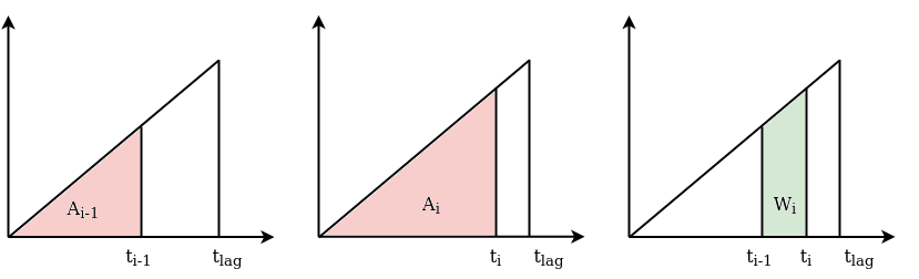
The half-triangular lag function grows linearly until \(t_{\textrm{lag}}\) and then drops to zero, as shown in the schematic. The slope \(\alpha\) is determined from the constraint that the total area of the triangle must be equal to 1.
SuperflexPy provides the class LagElement that contains most of the
functionalities needed to calculate the output of a lag function. The class
implementing a customized lag function will inherit from LagElement, and
implement only the methods needed to compute the weight array.
1import numpy as np
2
3class TriangularLag(LagElement):
The only method requiring implementation is the private method used to
calculate the weight array.
 1    def _build_weight(self, lag_time):
 2
 3        weight = []
 4
 5        for t in lag_time:
 6            array_length = np.ceil(t)
 7            w_i = []
 8
 9            for i in range(int(array_length)):
10                w_i.append(self._calculate_lag_area(i + 1, t)
11                           - self._calculate_lag_area(i, t))
12
13            weight.append(np.array(w_i))
14
15        return weight
The method _build_weight makes use of a secondary private static method
 1    @staticmethod
 2    def _calculate_lag_area(bin, len):
 3
 4        if bin <= 0:
 5            value = 0
 6        elif bin < len:
 7            value = (bin / len)**2
 8        else:
 9            value = 1
10
11        return value
This method returns the area \(A_i\) of the red triangle in the figure,
which has base \(t_i\) (bin). The method _build_weight uses
this function to calculate the weight array \(W_i\), as the difference
between \(A_i\) and \(A_{i-1}\).
Note that the method _build_weight can be implemented using other
approaches, e.g., without using auxiliary methods.
Parameterized splitter
A splitter is an element that takes the flux from an upstream element and distributes it to feed multiple downstream elements. The element is controlled by parameters that define the portions of the flux that go into specific elements.
The simple case that we consider here has a single input flux that is split to two downstream elements. In this case, the splitter requires only one parameter \(\alpha_{\textrm{split}}\). The fluxes to the downstream elements are
SuperflexPy provides the class ParameterizedElement, which can be
extended to implement all elements that are controlled by parameters but do not
have a state. The class implementing the parameterized splitter will inherit
from ParameterizedElement and implement only the methods required for
the new functionality.
1from superflexpy.framework.element import ParameterizedElement
2
3class ParameterizedSingleFluxSplitter(ParameterizedElement):
First, we define two private attributes that specify the number of upstream and downstream elements of the splitter. This information is used by the unit when constructing the model structure.
1    _num_downstream = 2
2    _num_upstream = 1
We then define the method that receives the inputs, and the method that calculates the outputs.
 1    def set_input(self, input):
 2
 3        self.input = {'Q_in': input[0]}
 4
 5    def get_output(self, solve=True):
 6
 7        split_par = self._parameters[self._prefix_parameters + 'split-par']
 8
 9        return [
10            self.input['Q_in'] * split_par,
11            self.input['Q_in'] * (1 - split_par)
12        ]
The two methods have the same structure as the ones implemented as part of the earlier
Linear reservoir example. Note that, in this case, the argument
solve of the method get_output is not used, but is still required to
maintain a consistent interface.