Note
Last update 23/08/2021
Numerical implementation
Reservoirs are the most common elements in conceptual hydrological models. Reservoirs are controlled by one (or more) ordinary differential equations (ODEs) of the form
and associated initial conditions.
Such differential equations are usually difficult or impossible to solve analytically, therefore, numerical methods are employed. These numerical methods take the form of time stepping schemes.
Available numerical routines to facilitate the solution of ODEs
The current implementation of SuperflexPy conceptualizes the solution of the ODE as a two-step procedure:
Construct the discrete-time equations defining the numerical approximation of the ODEs at a single time step, e.g. using Euler methods.
Solve the numerical approximation for the storage(s). This step usually require some iterative procedure since the algebraic equations resulting from point 1 are usually implicit.
These steps can be performed extending two SuperflexPy components:
NumericalApproximator and RootFinder.
SuperflexPy provides three built-in numerical approximators (implicit and explicit Euler, Runge Kutta 4) and a three root finders (one implementing the Pegasus method, one the Newton method, and one for explicit algebraic equations).
The suggested configuration, used in several modelling studies with the SUPERFLEX framework, is to use the Implicit Euler approximation and the Pegasus root finder. This setup, together with a “one-element-at-a-time” strategy to solve the elements, enables a very robust solution of the ODEs, since the numerical routines operate on a single ODE at a time. In such cases, the root finder also operates on a single algebraic equation at a time. Moreover, the Pegasus root finder implements bracketing methods, which are guaranteed to converge (to a tolerance within the common constraints of floating point arithmetic) as long as the initial solution bounds are known. The Pegasus algorithm is a bracket-based nonlinear solver similar to the well-known Regula Falsi algorithm. It employs a re-scaling of function values at the bracket endpoints to accelerate convergence for strongly curved functions. The authors of the paper (Dowell and Jarratt, 1972) claim that the algorithm exhibit superior asymptotic convergence properties to other modified linear methods.
In order to facilitate the convergence of the root finders and to reduce problems in calibration, we suggest to use smooth flux functions when implementing the elements (see Kavetski and Kuczera, 2007). If a user wants to experiment with discontinuous flux function, specific ODE solution algorithms should be carefully selected.
The following sections describe how to implement extensions of the classes
NumericalApproximator and RootFinder and how to write solver that
interfaces directly with the ODEsElement, bypassing the current architecture.
Creating a customized numerical approximator
A customized numerical approximator can be implemented by extending the class
NumericalApproximator and implementing two methods: _get_fluxes
and _differential_equation.
 1class CustomNumericalApproximator(NumericalApproximator):
 2
 3    @staticmethod
 4    def _get_fluxes(fluxes_fun, S, S0, args, dt):
 5
 6        # Some code here
 7
 8        return fluxes
 9
10    @staticmethod
11    def _differential_equation(fluxes_fun, S, S0, dt, args, ind):
12
13        # Some code here
14
15        return [diff_eq, min_val, max_val, d_diff_eq]
where fluxes_fun is a list of functions used to calculate the fluxes and their derivatives,
S is the state that solves the ODE, S0 is the initial state,
dt is the time step, args is a list of additional arguments used
by the functions in fluxes_fun, and ind is the index of the input
arrays to use.
The method _get_fluxes is responsible for calculating the fluxes after
the ODE has been solved. This method operates with a vector of states.
The method _differential_equation calculates the approximation of the
ODE. It returns the residual of the approximated mass balance equations for a
given value of S, the minimum and maximum bounds for the
search of the solution, and the value of the derivative of the residual of the approximated mass balance equations for a
given value of S w.r.t. S. This method is designed to be interfaced with the root
finder.
For further details, please see the implementation of Implicit and Explicit Euler.
Creating a customized root finder
A customized root finder can constructed by extending the class
RootFinder implementing the method solve.
1class CustomRootFinder(RootFinder):
2
3    def solve(self, diff_eq_fun, fluxes_fun, S0, dt, ind, args):
4
5        # Some code here
6
7        return root
where diff_eq_fun is a function that calculates the value of the
approximated ODE, fluxes_fun is a list of functions used to calculate
the fluxes and their derivatives, S0 is the initial state, dt is the time step,
args is a list of additional arguments used by the functions in
fluxes_fun, and ind is the index of the input arrays to use.
The method solve is responsible for finding the numerical solution of
the approximated ODE. In case of failure, the method should either raise a
RuntimeError (Python implementation) or return numpy.nan (this
is not ideal but it is the suggested workaround because Numba does not support
exceptions handling).
To understand better how the method solve works, please see the
implementation of the Pegasus and of the Newton root finders that are currently used in the SuperflexPy
applications.
Building a numerical solver from scratch
When implementing more advanced numerical schemes, the usage of NumericalApproximator
and RootFinder may be limiting. One example may be when the user wants
to use a numerical solver from an existing library.
In this case the user has to implement a new class from scratch that implements a solve
and a get_fluxes method. This class interfaces directly with the ODEsElement and
substitutes the combined usage of NumericalApproximator and RootFinder.
 1class CustomODESolver():
 2
 3    # The class may implement other methods
 4
 5    def solve(self, fluxes_fun, S0, dt, args):
 6
 7        # Some code here
 8
 9        return states
10
11    def get_fluxes(self, fluxes_fun, S, S0, dt, args):
12
13        # Some code here
14
15        return fluxes
where fluxes_fun is a list of functions used to calculate
the fluxes and their derivatives, S0 is the initial state, dt is the time step,
args is a list of additional arguments used by the functions in
fluxes_fun (e.g, input fluxes, parameters, etc), and S is this the state of the reservoir.
The solve method is responsible for “assembling” and solving the differential
equations and their derivatives. The fluxes controlling the differential equations can be calculated,
for any possible state and parameters, using the functions contained in
fluxes_fun, which are implemented in the single ODEsElement.
The method returns an array (time series) containing the values of the states
according to the time step dt. It is important to notice that nothing
forbids to calculate the states at intermediate time steps, keeping in mind
the additional error introduced by considering the fluxes constant over dt
(see Sequential solution of the elements and numerical approximations).
The get_fluxes method is responsible for calculating the fluxes, once
the ODEs have already been solved.
SuperflexPy does not implement functioning customized ODEs solvers created from scratch (e.g.,
encapsulating the functionality of external libraries). However, to understand
better how to implement a custom ODEs solver from scratch the user can have a
look at the implementation of the abstract class NumericalApproximator,
which represents itself an ODEs solver implemented from scratch.
Sequential solution of the elements and numerical approximations
The SuperflexPy framework is built on a model representation that maps to a directional acyclic graph. Model elements are solved sequentially from upstream to downstream, with the output from each element being used as input to its downstream elements.
Moreover, inputs and outputs of the elements are considered constant over the
time step dt whereas in reality fluxes vary within the time step; this
choice simplifies the implementation of the framework and is coherent with the
typical format of forcing data such as rainfall, PET, etc, which is tabulated in
discrete steps.
When fixed-step solvers are used (e.g. implicit Euler), this “one-element-at-a-time” strategy is equivalent to applying the same (fixed-step) solver to the entire ODE system simultaneously (i.e., no additional approximation error is introduced), as fixed-step solvers transform the ODE system into a lower triangular system of nonlinear algebraic equations, which can be solved using forward elimination. The usage of constant fluxes does not introduce approximations in this case, since intermediate fluxes are not needed.
However, when solvers with internal substepping are used, the “constant fluxes” choice introduces additional approximation error, since solvers cannot access the actual value of the fluxes within the time step but only their approximation to the average value.
These numerical approximations could be removed only by the coupled solution of the ODEs system. Alternative solutions could be adopted to reduce the approximation, while respecting the “one-element-at-a-time” strategy; one option could be, for the elements to output instead of a single number, an array of values, or a function, or a specific data structure that allows for returning the values at intermediate time steps. However, all the possibilities listed in this paragraph are currently not supported by SuperflexPy and not foreseen as development in the near future.
Computational efficiency with Numpy and Numba
Conceptual hydrological models are often used in computationally demanding contexts, such as parameter calibration and uncertainty quantification, which require many model runs (thousands or even millions). Computational efficiency is therefore an important requirement of SuperflexPy.
Computational efficiency is a potential limitation of pure Python, but libraries like Numpy and Numba can help in pushing the performance closer to traditionally fast languages such as Fortran and C.
Numpy provides highly efficient arrays for vectorized operations (i.e. elementwise operations between arrays). Numba provides a “just-in-time compiler” that can be used to compile (at runtime) a normal Python method to machine code that operates efficiently with Numpy arrays. The combined use of Numpy and Numba is extremely effective when solving ODEs using time stepping schemes, where the method loops through a vector to perform elementwise operations.
SuperflexPy includes Numba-optimized versions of
NumericalApproximator and RootFinder, which enable efficient
solution of ODEs describing the reservoir elements.
The figure below compares the execution times of pure Python vs. the Numba implementation, as a function of the length of the time series (upper panel) and the number of model runs (lower panel). Simulations were run on a laptop (single thread), using the HYMOD model, solved using the implicit Euler numerical solver.
The plot clearly shows the tradeoff between compilation time (which is zero for Python and around 2 seconds for Numba) versus run time (where Numba is 30 times faster than Python). For example, a single run of 1000 time steps takes 0.11 seconds with Python and 1.85 seconds with Numba. In contrast, if the same model is run 100 times (e.g., as part of a calibration) the Python version takes 11.75 seconds while the Numba version takes 2.35 seconds.
Note
The objective of these plots is to give an idea of time that is topically required to perform common modelling applications (e.g., calibration) with SuperflexPy, to show the impact of the Numba implementation, and to explain the tradeoff between compilation and run time. The results do not have to be considered as accurate measurements of the performance of SuperflexPy (i.e., rigorous benchmarking).
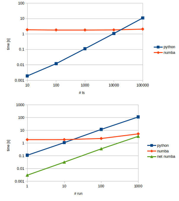
The green line “net numba” in the lower panel express the run time of the Numba implementation, i.e., excluding the compilation time.