Note
Last update 01/09/2020
Application: implementation of existing conceptual models
In this page we propose the implementation of existing conceptual hydrological models. The translation of a model in SuperflexPy requires the following steps:
- Design of a structure that reflects the original model but satisfy the requirements of SuperflexPy (e.g. does not contain mutual interaction between elements);
- Extension of the framework, coding the required elements (as explained in the page Expand SuperflexPy: build customized elements)
- Construction of the model structure using the elements implemented at point 2
M4 from Kavetski and Fenicia, WRR, 2011
M4 is a simple conceptual model presented, as part of a models comparison study, in the article
Kavetski, D., and F. Fenicia (2011), Elements of a flexible approach for conceptual hydrological modeling: 2. Applicationand experimental insights, WaterResour.Res.,47, W11511, doi:10.1029/2011WR010748.
Design of the structure
The structure of M4 is quite simple and can be implemented directly in SuperflexPy without the need of using connection elements. The figure shows, on the left, the structure as shown in the paper and, on the right, the SuperflexPy implementation. as part of a models comparison study.
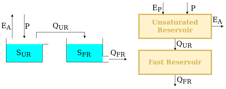
The upstream element, the unsaturated reservoir (UR), is designed to represent runoff generation processes (e.g. separation between evaporation and runoff) and it is controlled by the differential equation
The downstream element, the fast reservoir (FR), is designed to represent runoff propagation processes (e.g. routing) and it is controlled by the differential equation
\(S_{\textrm{UR}}\) and \(S_{\textrm{FR}}\) are the states of the reservoirs, \(P\) is the input flux, \(E_{\textrm{P}}\) is the potential evapotranspiration, and \(S_{\textrm{max}}\), \(m\), \(\beta\), \(k\), \(\alpha\) are parameters of the model.
Elements creation
We now report the code used to implement the elements designed in the previous section. Instruction on how to use the framework to build new elements can be found in the page Expand SuperflexPy: build customized elements.
Note that for common applications the elements are already available (refer to the page Elements list) and, therefore, the modeller does not need to implement the code presented in this section.
Unsaturated reservoir
The element is a reservoir that can be implemented extending the
ODEsElement class.
1 2 3 4 5 6 7 8 9 10 11 12 13 14 15 16 17 18 19 20 21 22 23 24 25 26 27 28 29 30 31 32 33 34 35 36 37 38 39 40 41 42 43 44 45 46 47 48 49 50 51 52 53 54 55 56 57 58 59 60 61 62 63 64 65 66 67 68 69 70 71 72 73 74 75 76 77 78 79 80 81 82 83 84 85 86 87 88 89 90 91 92 93 94 95 96 97 98 99 | class UnsaturatedReservoir(ODEsElement):
def __init__(self, parameters, states, approximation, id):
ODEsElement.__init__(self,
parameters=parameters,
states=states,
approximation=approximation,
id=id)
self._fluxes_python = [self._fluxes_function_python]
if approximation.architecture == 'numba':
self._fluxes = [self._fluxes_function_numba]
elif approximation.architecture == 'python':
self._fluxes = [self._fluxes_function_python]
def set_input(self, input):
self.input = {'P': input[0],
'PET': input[1]}
def get_output(self, solve=True):
if solve:
self._solver_states = [self._states[self._prefix_states + 'S0']]
self._solve_differential_equation()
# Update the state
self.set_states({self._prefix_states + 'S0': self.state_array[-1, 0]})
fluxes = self._num_app.get_fluxes(fluxes=self._fluxes_python,
S=self.state_array,
S0=self._solver_states,
**self.input,
**{k[len(self._prefix_parameters):]: self._parameters[k] for k in self._parameters},
)
return [-fluxes[0][2]]
def get_AET(self):
try:
S = self.state_array
except AttributeError:
message = '{}get_aet method has to be run after running '.format(self._error_message)
message += 'the model using the method get_output'
raise AttributeError(message)
fluxes = self._num_app.get_fluxes(fluxes=self._fluxes_python,
S=S,
S0=self._solver_states,
**self.input,
**{k[len(self._prefix_parameters):]: self._parameters[k] for k in self._parameters},
)
return [- fluxes[0][1]]
# PROTECTED METHODS
@staticmethod
def _fluxes_function_python(S, S0, ind, P, Smax, m, beta, PET):
if ind is None:
return (
[
P,
- PET * ((S / Smax) * (1 + m)) / ((S / Smax) + m),
- P * (S / Smax)**beta,
],
0.0,
S0 + P
)
else:
return (
[
P[ind],
- PET[ind] * ((S / Smax[ind]) * (1 + m[ind])) / ((S / Smax[ind]) + m[ind]),
- P[ind] * (S / Smax[ind])**beta[ind],
],
0.0,
S0 + P[ind]
)
@staticmethod
@nb.jit('Tuple((UniTuple(f8, 3), f8, f8))(optional(f8), f8, i4, f8[:], f8[:], f8[:], f8[:], f8[:])',
nopython=True)
def _fluxes_function_numba(S, S0, ind, P, Smax, m, beta, PET):
return (
(
P[ind],
PET[ind] * ((S / Smax[ind]) * (1 + m[ind])) / ((S / Smax[ind]) + m[ind]),
- P[ind] * (S / Smax[ind])**beta[ind],
),
0.0,
S0 + P[ind]
)
|
Fast reservoir
The element is a reservoir that can be implemented extending the
ODEsElement class.
1 2 3 4 5 6 7 8 9 10 11 12 13 14 15 16 17 18 19 20 21 22 23 24 25 26 27 28 29 30 31 32 33 34 35 36 37 38 39 40 41 42 43 44 45 46 47 48 49 50 51 52 53 54 55 56 57 58 59 60 61 62 63 64 65 66 67 68 69 70 71 72 73 74 75 76 77 78 | class FastReservoir(ODEsElement):
def __init__(self, parameters, states, approximation, id):
ODEsElement.__init__(self,
parameters=parameters,
states=states,
approximation=approximation,
id=id)
self._fluxes_python = [self._fluxes_function_python] # Used by get fluxes, regardless of the architecture
if approximation.architecture == 'numba':
self._fluxes = [self._fluxes_function_numba]
elif approximation.architecture == 'python':
self._fluxes = [self._fluxes_function_python]
# METHODS FOR THE USER
def set_input(self, input):
self.input = {'P': input[0]}
def get_output(self, solve=True):
if solve:
self._solver_states = [self._states[self._prefix_states + 'S0']]
self._solve_differential_equation()
# Update the state
self.set_states({self._prefix_states + 'S0': self.state_array[-1, 0]})
fluxes = self._num_app.get_fluxes(fluxes=self._fluxes_python, # I can use the python method since it is fast
S=self.state_array,
S0=self._solver_states,
**self.input,
**{k[len(self._prefix_parameters):]: self._parameters[k] for k in self._parameters},
)
return [- fluxes[0][1]]
# PROTECTED METHODS
@staticmethod
def _fluxes_function_python(S, S0, ind, P, k, alpha):
if ind is None:
return (
[
P,
- k * S**alpha,
],
0.0,
S0 + P
)
else:
return (
[
P[ind],
- k[ind] * S**alpha[ind],
],
0.0,
S0 + P[ind]
)
@staticmethod
@nb.jit('Tuple((UniTuple(f8, 2), f8, f8))(optional(f8), f8, i4, f8[:], f8[:], f8[:])',
nopython=True)
def _fluxes_function_numba(S, S0, ind, P, k, alpha):
return (
(
P[ind],
- k[ind] * S**alpha[ind],
),
0.0,
S0 + P[ind]
)
|
Model initialization
Now that all the elements needed have been implemented, we can put them together to build the model structure. For details refer to Quick demo.
The first step consists in initializing all the elements.
1 2 3 4 5 6 7 8 9 10 11 12 13 14 15 16 | root_finder = PegasusPython()
numeric_approximator = ImplicitEulerPython(root_finder=root_finder)
ur = UnsaturatedReservoir(
parameters={'Smax': 50.0, 'Ce': 1.0, 'm': 0.01, 'beta': 2.0},
states={'S0': 25.0},
approximation=numeric_approximator,
id='UR'
)
fr = FastReservoir(
parameters={'k': 0.1, 'alpha': 1.0},
states={'S0': 10.0},
approximation=numeric_approximator,
id='FR'
)
|
After that, the elements can be put together to create a Unit that
reflects the structure presented in the figure.
1 2 3 4 5 6 7 | model = Unit(
layers=[
[ur],
[fr]
],
id='M4'
)
|
GR4J
GR4J is a conceptual hydrological model originally introduced in the article
Perrin, C., Michel, C., and Andréassian, V.: Improvement of a parsimonious model for streamflow simulation, Journal of Hydrology, 279, 275-289, https://doi.org/10.1016/S0022-1694(03)00225-7, 2003.
The solution adopted here follows the “continuous state-space representation” presented in
Santos, L., Thirel, G., and Perrin, C.: Continuous state-space representation of a bucket-type rainfall-runoff model: a case study with the GR4 model using state-space GR4 (version 1.0), Geosci. Model Dev., 11, 1591-1605, 10.5194/gmd-11-1591-2018, 2018.
Design of the structure
The figure shows, on the left, the model structure as proposed in Perrin et al., 2003 and, on the right, the adaptation to SuperflexPy
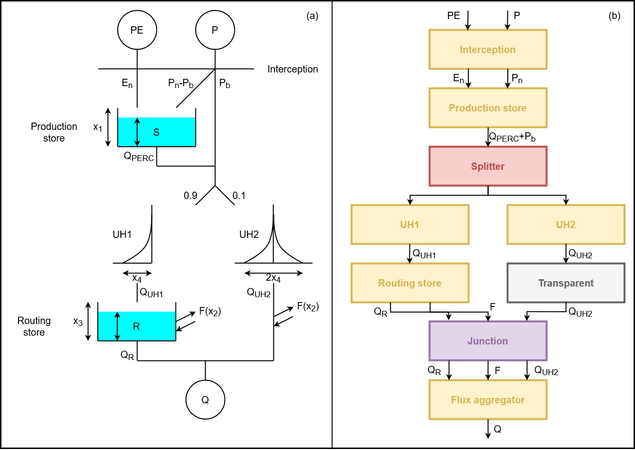
In the original version, the potential evaporation and the precipitation are “filtered” by an interception layer that sets the smallest of the two fluxes to zero and the biggest to the difference between the two.
This element is reproduced identically in the SuperflexPy implementation by the “interception filter”
In the original model, the precipitation is split between a portion \(P_s\) that flows into the production store and the remaining part \(P_b\) that bypasses the reservoir. Since \(P_s\) and \(P_b\) are function of the state of the reservoir
when we implement this part of the model in SuperflexPy, these two fluxes cannot be calculated before solving the reservoir. For this reason, in the SuperflexPy implementation of GR4J, all the precipitation flows into an element that incorporates the production store; this element takes care of dividing the precipitation internally, while solving the differential equation
where the first term is the precipitation \(P_s\), the second term is the actual evaporation, and the third term represent the output of the reservoir, called “percolation”.
Once the reservoir is solved (i.e. the values of \(S_{\textrm{UR}}\) that solve the differential equation are found), the element outputs the sum of percolation and bypassing precipitation \(P_b\)
After this, the flux is divided between two lag functions (called “unit hydrograph”, abbreviated UH): 90% of the flux goes to UH1 while the 10% goes to UH2. In this part of the structure there is a strict correspondence between the elements of GR4J and their SuperflexPy implementation.
The output of UH1 represents the input of the routing store, a reservoir that is controlled by the differential equation
where the second term is the output of the reservoir and the last is a gain/loss term (called \(Q_{\textrm{RF}}\)).
The gain/loss term \(Q_{\textrm{RF}}\), which is a function of the state \(S_{\textrm{RR}}\) of the reservoir, is subtracted also to the output of UH2: in SuperflexPy, this operation cannot be done together with the solution of the routing store but it is done afterwards. For this reason, the SuperflexPy implementation of GR4J has an additional element (called “flux aggregator”) that collects (through a junction element) the output of the routing store, the gain/loss term, and the output of UH2 and computes the outflow of the model using the equation
Elements creation
We now report the code used to implement the elements designed in the previous section. Instruction on how to use the framework to build new elements can be found in the page Expand SuperflexPy: build customized elements.
Note that for common applications the elements are already available (refer to the page Elements list) and, therefore, the modeller does not need to implement the code presented in this section.
Interception
The interception filter can be implemented extending the class
BaseElement
1 2 3 4 5 6 7 8 9 10 11 12 13 14 15 16 | class InterceptionFilter(BaseElement):
_num_upstream = 1
_num_downstream = 1
def set_input(self, input):
self.input = {}
self.input['PET'] = input[0]
self.input['P'] = input[1]
def get_output(self, solve=True):
remove = np.minimum(self.input['PET'], self.input['P'])
return [self.input['PET'] - remove, self.input['P'] - remove]
|
Production store
The production store is controlled by a differential equation and, therefore,
it can be constructed extending the class ODEsElement
1 2 3 4 5 6 7 8 9 10 11 12 13 14 15 16 17 18 19 20 21 22 23 24 25 26 27 28 29 30 31 32 33 34 35 36 37 38 39 40 41 42 43 44 45 46 47 48 49 50 51 52 53 54 55 56 57 58 59 60 61 62 63 64 65 66 67 68 69 70 71 72 73 74 75 76 77 78 79 80 81 82 83 84 85 86 87 88 89 90 91 92 93 94 95 96 97 98 99 100 101 102 | class ProductionStore(ODEsElement):
def __init__(self, parameters, states, approximation, id):
ODEsElement.__init__(self,
parameters=parameters,
states=states,
approximation=approximation,
id=id)
self._fluxes_python = [self._flux_function_python]
if approximation.architecture == 'numba':
self._fluxes = [self._flux_function_numba]
elif approximation.architecture == 'python':
self._fluxes = [self._flux_function_python]
def set_input(self, input):
self.input = {}
self.input['PET'] = input[0]
self.input['P'] = input[1]
def get_output(self, solve=True):
if solve:
# Solve the differential equation
self._solver_states = [self._states[self._prefix_states + 'S0']]
self._solve_differential_equation()
# Update the states
self.set_states({self._prefix_states + 'S0': self.state_array[-1, 0]})
fluxes = self._num_app.get_fluxes(fluxes=self._fluxes_python,
S=self.state_array,
S0=self._solver_states,
dt=self._dt,
**self.input,
**{k[len(self._prefix_parameters):]: self._parameters[k] for k in self._parameters},
)
Pn_minus_Ps = self.input['P'] - fluxes[0][0]
Perc = - fluxes[0][2]
return [Pn_minus_Ps + Perc]
def get_aet(self):
try:
S = self.state_array
except AttributeError:
message = '{}get_aet method has to be run after running '.format(self._error_message)
message += 'the model using the method get_output'
raise AttributeError(message)
fluxes = self._num_app.get_fluxes(fluxes=self._fluxes_python,
S=S,
S0=self._solver_states,
dt=self._dt,
**self.input,
**{k[len(self._prefix_parameters):]: self._parameters[k] for k in self._parameters},
)
return [- fluxes[0][1]]
@staticmethod
def _flux_function_python(S, S0, ind, P, x1, alpha, beta, ni, PET, dt):
if ind is None:
return(
[
P * (1 - (S / x1)**alpha), # Ps
- PET * (2 * (S / x1) - (S / x1)**alpha), # Evaporation
- ((x1**(1 - beta)) / ((beta - 1) * dt)) * (ni**(beta - 1)) * (S**beta) # Perc
],
0.0,
S0 + P * (1 - (S / x1)**alpha)
)
else:
return(
[
P[ind] * (1 - (S / x1[ind])**alpha[ind]), # Ps
- PET[ind] * (2 * (S / x1[ind]) - (S / x1[ind])**alpha[ind]), # Evaporation
- ((x1[ind]**(1 - beta[ind])) / ((beta[ind] - 1) * dt[ind])) * (ni[ind]**(beta[ind] - 1)) * (S**beta[ind]) # Perc
],
0.0,
S0 + P[ind] * (1 - (S / x1[ind])**alpha[ind])
)
@staticmethod
@nb.jit('Tuple((UniTuple(f8, 3), f8, f8))(optional(f8), f8, i4, f8[:], f8[:], f8[:], f8[:], f8[:], f8[:], f8[:])',
nopython=True)
def _flux_function_numba(S, S0, ind, P, x1, alpha, beta, ni, PET, dt):
return(
(
P[ind] * (1 - (S / x1[ind])**alpha[ind]), # Ps
- PET[ind] * (2 * (S / x1[ind]) - (S / x1[ind])**alpha[ind]), # Evaporation
- ((x1[ind]**(1 - beta[ind])) / ((beta[ind] - 1) * dt[ind])) * (ni[ind]**(beta[ind] - 1)) * (S**beta[ind]) # Perc
),
0.0,
S0 + P[ind] * (1 - (S / x1[ind])**alpha[ind])
)
|
Unit hydrographs
The unit hydrographs are an extension of the LagElement and they can
be implemented with the following code
1 2 3 4 5 6 7 8 9 10 11 12 13 14 15 16 17 18 19 20 21 22 23 24 25 26 27 28 29 | class UnitHydrograph1(LagElement):
def __init__(self, parameters, states, id):
LagElement.__init__(self, parameters, states, id)
def _build_weight(self, lag_time):
weight = []
for t in lag_time:
array_length = np.ceil(t)
w_i = []
for i in range(int(array_length)):
w_i.append(self._calculate_lag_area(i + 1, t)
- self._calculate_lag_area(i, t))
weight.append(np.array(w_i))
return weight
@staticmethod
def _calculate_lag_area(bin, len):
if bin <= 0:
value = 0
elif bin < len:
value = (bin / len)**2.5
else:
value = 1
return value
|
1 2 3 4 5 6 7 8 9 10 11 12 13 14 15 16 17 18 19 20 21 22 23 24 25 26 27 28 29 30 31 32 | class UnitHydrograph2(LagElement):
def __init__(self, parameters, states, id):
LagElement.__init__(self, parameters, states, id)
def _build_weight(self, lag_time):
weight = []
for t in lag_time:
array_length = np.ceil(t)
w_i = []
for i in range(int(array_length)):
w_i.append(self._calculate_lag_area(i + 1, t)
- self._calculate_lag_area(i, t))
weight.append(np.array(w_i))
return weight
@staticmethod
def _calculate_lag_area(bin, len):
half_len = len / 2
if bin <= 0:
value = 0
elif bin < half_len:
value = 0.5 * (bin / half_len)**2.5
elif bin < len:
value = 1 - 0.5 * (2 - bin / half_len)**2.5
else:
value = 1
return value
|
Routing store
The routing store is an ODEsElement
1 2 3 4 5 6 7 8 9 10 11 12 13 14 15 16 17 18 19 20 21 22 23 24 25 26 27 28 29 30 31 32 33 34 35 36 37 38 39 40 41 42 43 44 45 46 47 48 49 50 51 52 53 54 55 56 57 58 59 60 61 62 63 64 65 66 67 68 69 70 71 72 73 74 75 76 77 78 79 80 81 82 83 | class RoutingStore(ODEsElement):
def __init__(self, parameters, states, approximation, id):
ODEsElement.__init__(self,
parameters=parameters,
states=states,
approximation=approximation,
id=id)
self._fluxes_python = [self._flux_function_python]
if approximation.architecture == 'numba':
self._fluxes = [self._flux_function_numba]
elif approximation.architecture == 'python':
self._fluxes = [self._flux_function_python]
def set_input(self, input):
self.input = {}
self.input['P'] = input[0]
def get_output(self, solve=True):
if solve:
# Solve the differential equation
self._solver_states = [self._states[self._prefix_states + 'S0']]
self._solve_differential_equation()
# Update the states
self.set_states({self._prefix_states + 'S0': self.state_array[-1, 0]})
fluxes = self._num_app.get_fluxes(fluxes=self._fluxes_python,
S=self.state_array,
S0=self._solver_states,
dt=self._dt,
**self.input,
**{k[len(self._prefix_parameters):]: self._parameters[k] for k in self._parameters},
)
Qr = - fluxes[0][1]
F = -fluxes[0][2]
return [Qr, F]
@staticmethod
def _flux_function_python(S, S0, ind, P, x2, x3, gamma, omega, dt):
if ind is None:
return(
[
P, # P
- ((x3**(1 - gamma)) / ((gamma - 1) * dt)) * (S**gamma), # Qr
- (x2 * (S / x3)**omega), # F
],
0.0,
S0 + P
)
else:
return(
[
P[ind], # P
- ((x3[ind]**(1 - gamma[ind])) / ((gamma[ind] - 1) * dt[ind])) * (S**gamma[ind]), # Qr
- (x2[ind] * (S / x3[ind])**omega[ind]), # F
],
0.0,
S0 + P[ind]
)
@staticmethod
@nb.jit('Tuple((UniTuple(f8, 3), f8, f8))(optional(f8), f8, i4, f8[:], f8[:], f8[:], f8[:], f8[:], f8[:])',
nopython=True)
def _flux_function_numba(S, S0, ind, P, x2, x3, gamma, omega, dt):
return(
(
P[ind], # P
- ((x3[ind]**(1 - gamma[ind])) / ((gamma[ind] - 1) * dt[ind])) * (S**gamma[ind]), # Qr
- (x2[ind] * (S / x3[ind])**omega[ind]), # F
),
0.0,
S0 + P[ind]
)
|
Flux aggregator
The flux aggregator can be implemented extending a BaseElement
1 2 3 4 5 6 7 8 9 10 11 12 13 14 15 16 | class FluxAggregator(BaseElement):
_num_downstream = 1
_num_upstream = 1
def set_input(self, input):
self.input = {}
self.input['Qr'] = input[0]
self.input['F'] = input[1]
self.input['Q2_out'] = input[2]
def get_output(self, solve=True):
return [self.input['Qr']
+ np.maximum(0, self.input['Q2_out'] - self.input['F'])]
|
Model initialization
Now that all the elements needed have been implemented, we can put them together to build the model structure. For details refer to Quick demo.
The first step consists in initializing all the elements.
1 2 3 4 5 6 7 8 9 10 11 12 13 14 15 16 17 18 19 20 21 22 23 24 25 26 27 28 29 30 31 32 33 34 35 36 37 38 39 | x1, x2, x3, x4 = (50.0, 0.1, 20.0, 3.5)
root_finder = PegasusPython() # Use the default parameters
numerical_approximation = ImplicitEulerPython(root_finder)
interception_filter = InterceptionFilter(id='ir')
production_store = ProductionStore(parameters={'x1': x1, 'alpha': 2.0,
'beta': 5.0, 'ni': 4/9},
states={'S0': 10.0},
approximation=numerical_approximation,
id='ps')
splitter = Splitter(weight=[[0.9], [0.1]],
direction=[[0], [0]],
id='spl')
unit_hydrograph_1 = UnitHydrograph1(parameters={'lag-time': x4},
states={'lag': None},
id='uh1')
unit_hydrograph_2 = UnitHydrograph2(parameters={'lag-time': 2*x4},
states={'lag': None},
id='uh2')
routing_store = RoutingStore(parameters={'x2': x2, 'x3': x3,
'gamma': 5.0, 'omega': 3.5},
states={'S0': 10.0},
approximation=numerical_approximation,
id='rs')
transparent = Transparent(id='tr')
junction = Junction(direction=[[0, None], # First output
[1, None], # Second output
[None, 0]], # Third output
id='jun')
flux_aggregator = FluxAggregator(id='fa')
|
After that, the elements can be put together to create a Unit that
reflects the structure presented in the figure.
1 2 3 4 5 6 7 8 | model = Unit(layers=[[interception_filter],
[production_store],
[splitter],
[unit_hydrograph_1, unit_hydrograph_2],
[routing_store, transparent],
[junction],
[flux_aggregator]],
id='model')
|
HYMOD
HYMOD is a conceptual hydrological model presented in the Ph.D. thesis
Boyle, D. P. (2001). Multicriteria calibration of hydrologic models, The University of Arizona. Link
The solution proposed here follows the model structure presented in
Wagener, T., Boyle, D. P., Lees, M. J., Wheater, H. S., Gupta, H. V., and Sorooshian, S.: A framework for development and application of hydrological models, Hydrol. Earth Syst. Sci., 5, 13–26, https://doi.org/10.5194/hess-5-13-2001, 2001.
Design of the structure
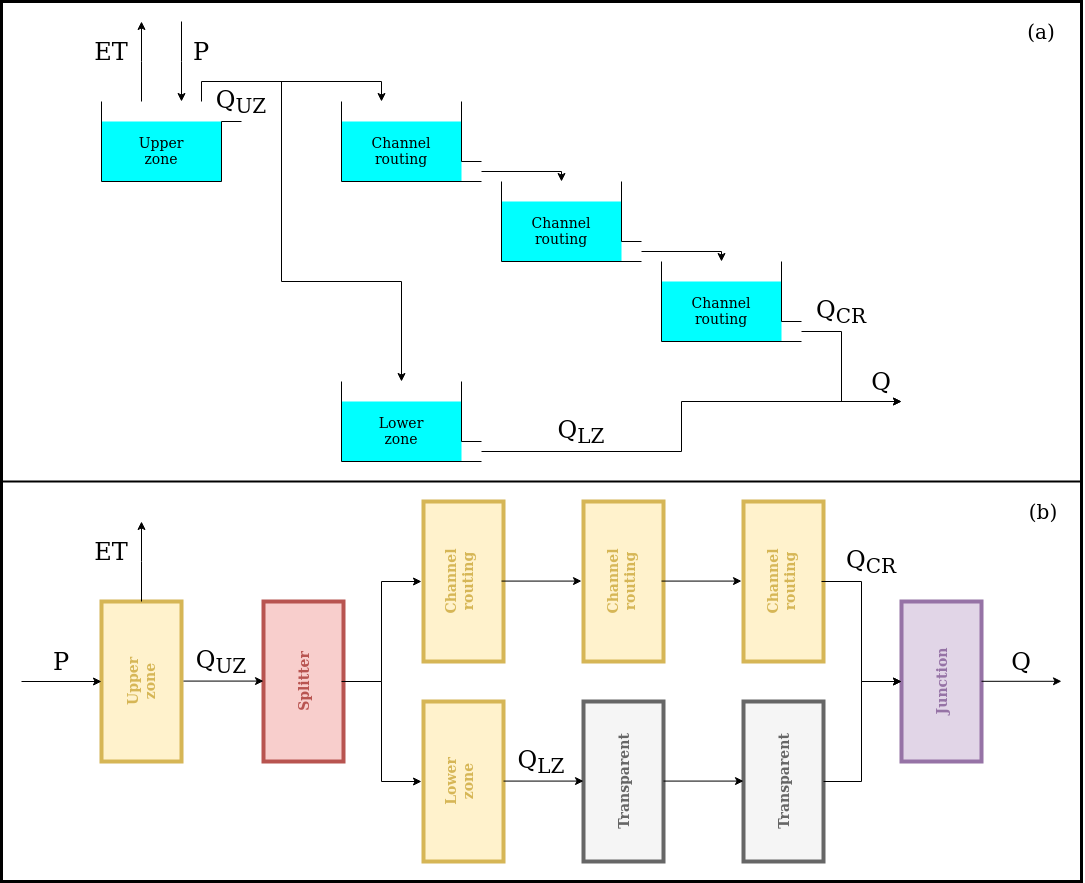
The structure of HYMOD is composed by three blocks of reservoirs that are designed to represent three mechanism that control the streamflow at the catchment scale: upper zone (soil dynamics), channel routing (surface runoff), and lower zone (subsurface flow).
As it can be seen in the figure, the original structure of HYMOD already satisfy the design constrains of SuperflexPy and therefore it can be implemented simply translating the single elements individually, without the need of workarounds, as done in the case of GR4J.
The first element (upper zone) is a reservoirs intended to represent soil dynamics that simulates streamflow generation processes and evaporation. It is controlled by the differential equation
where the first term represent the precipitation input, the second the actual evaporation (which is equal to the potential evaporation as long as there is sufficient storage in the reservoir) and the third the outflow of the reservoir.
The outflow of the reservoir is then split between the channel routing and the lower zone; these are all represented by some linear reservoirs that are controlled by the differential equation
where the first term is the input of the reservoir (the outflow of the upstream element, in this case) and the second term represent the outflow of the reservoir.
Channel routing and lower zone differentiate one from the other by two factors: the number of reservoirs used (3 in the first case and 1 in the second) and by the value of the parameter \(k\), which controls the outflow rate, that is bigger for the channel routing.
The output of these two branches of the model are collected together by a junction, which sums them to generate the output of the model.
Comparing the two panels in the figure, the only difference is due to the presence of the two transparent element that are needed to fill the gaps that, otherwise, will be present in the structure.
Elements creation
We now report the code used to implement the elements designed in the previous section. Instruction on how to use the framework to build new elements can be found in the page Expand SuperflexPy: build customized elements.
Note that for common applications the elements are already available (refer to the page Elements list) and, therefore, the modeller does not need to implement the code presented in this section.
Upper zone
The code used to simulate the upper zone present a change in the equation used to calculate the actual evaporation. In the original version (Wagener et al., 2001) the equation is “described” in the text
The actual evapotranspiration is equal to the potential value if sufficient soil moisture is available; otherwise it is equal to the available soil moisture content.
which translates to the equation
Unfortunately this solution is not smooth and this can cause some computational problems. For this reason, it has been decided to use the following equation to calculate the potential evaporation
The upper zone reservoir can be implemented extending the ODEsElement
class.
1 2 3 4 5 6 7 8 9 10 11 12 13 14 15 16 17 18 19 20 21 22 23 24 25 26 27 28 29 30 31 32 33 34 35 36 37 38 39 40 41 42 43 44 45 46 47 48 49 50 51 52 53 54 55 56 57 58 59 60 61 62 63 64 65 66 67 68 69 70 71 72 73 74 75 76 77 78 79 80 81 82 83 84 85 86 87 88 89 90 91 92 93 94 95 96 97 98 99 | class UpperZone(ODEsElement):
def __init__(self, parameters, states, approximation, id):
ODEsElement.__init__(self,
parameters=parameters,
states=states,
approximation=approximation,
id=id)
self._fluxes_python = [self._fluxes_function_python]
if approximation.architecture == 'numba':
self._fluxes = [self._fluxes_function_numba]
elif approximation.architecture == 'python':
self._fluxes = [self._fluxes_function_python]
def set_input(self, input):
self.input = {'P': input[0],
'PET': input[1]}
def get_output(self, solve=True):
if solve:
self._solver_states = [self._states[self._prefix_states + 'S0']]
self._solve_differential_equation()
# Update the state
self.set_states({self._prefix_states + 'S0': self.state_array[-1, 0]})
fluxes = self._num_app.get_fluxes(fluxes=self._fluxes_python,
S=self.state_array,
S0=self._solver_states,
**self.input,
**{k[len(self._prefix_parameters):]: self._parameters[k] for k in self._parameters},
)
return [-fluxes[0][2]]
def get_AET(self):
try:
S = self.state_array
except AttributeError:
message = '{}get_aet method has to be run after running '.format(self._error_message)
message += 'the model using the method get_output'
raise AttributeError(message)
fluxes = self._num_app.get_fluxes(fluxes=self._fluxes_python,
S=S,
S0=self._solver_states,
**self.input,
**{k[len(self._prefix_parameters):]: self._parameters[k] for k in self._parameters},
)
return [- fluxes[0][1]]
# PROTECTED METHODS
@staticmethod
def _fluxes_function_python(S, S0, ind, P, Smax, m, beta, PET):
if ind is None:
return (
[
P,
- PET * ((S / Smax) * (1 + m)) / ((S / Smax) + m),
- P * (1 - (1 - (S / Smax))**beta),
],
0.0,
S0 + P
)
else:
return (
[
P[ind],
- PET[ind] * ((S / Smax[ind]) * (1 + m[ind])) / ((S / Smax[ind]) + m[ind]),
- P[ind] * (1 - (1 - (S / Smax[ind]))**beta[ind]),
],
0.0,
S0 + P[ind]
)
@staticmethod
@nb.jit('Tuple((UniTuple(f8, 3), f8, f8))(optional(f8), f8, i4, f8[:], f8[:], f8[:], f8[:], f8[:])',
nopython=True)
def _fluxes_function_numba(S, S0, ind, P, Smax, m, beta, PET):
return (
(
P[ind],
- PET[ind] * ((S / Smax[ind]) * (1 + m[ind])) / ((S / Smax[ind]) + m[ind]),
- P[ind] * (1 - (1 - (S / Smax[ind]))**beta[ind]),
),
0.0,
S0 + P[ind]
)
|
Channel routing and lower zone
All the elements belonging to the channel routing and to the lower zone are
reservoirs that can be implemented extending the ODEsElement class.
1 2 3 4 5 6 7 8 9 10 11 12 13 14 15 16 17 18 19 20 21 22 23 24 25 26 27 28 29 30 31 32 33 34 35 36 37 38 39 40 41 42 43 44 45 46 47 48 49 50 51 52 53 54 55 56 57 58 59 60 61 62 63 64 65 66 67 68 69 70 71 72 73 74 75 76 77 78 | class LinearReservoir(ODEsElement):
def __init__(self, parameters, states, approximation, id):
ODEsElement.__init__(self,
parameters=parameters,
states=states,
approximation=approximation,
id=id)
self._fluxes_python = [self._fluxes_function_python] # Used by get fluxes, regardless of the architecture
if approximation.architecture == 'numba':
self._fluxes = [self._fluxes_function_numba]
elif approximation.architecture == 'python':
self._fluxes = [self._fluxes_function_python]
# METHODS FOR THE USER
def set_input(self, input):
self.input = {'P': input[0]}
def get_output(self, solve=True):
if solve:
self._solver_states = [self._states[self._prefix_states + 'S0']]
self._solve_differential_equation()
# Update the state
self.set_states({self._prefix_states + 'S0': self.state_array[-1, 0]})
fluxes = self._num_app.get_fluxes(fluxes=self._fluxes_python, # I can use the python method since it is fast
S=self.state_array,
S0=self._solver_states,
**self.input,
**{k[len(self._prefix_parameters):]: self._parameters[k] for k in self._parameters},
)
return [- fluxes[0][1]]
# PROTECTED METHODS
@staticmethod
def _fluxes_function_python(S, S0, ind, P, k):
if ind is None:
return (
[
P,
- k * S,
],
0.0,
S0 + P
)
else:
return (
[
P[ind],
- k[ind] * S,
],
0.0,
S0 + P[ind]
)
@staticmethod
@nb.jit('Tuple((UniTuple(f8, 2), f8, f8))(optional(f8), f8, i4, f8[:], f8[:])',
nopython=True)
def _fluxes_function_numba(S, S0, ind, P, k):
return (
(
P[ind],
- k[ind] * S,
),
0.0,
S0 + P[ind]
)
|
Model initialization
Now that all the elements needed have been implemented, we can put them together to build the model structure. For details refer to Quick demo.
The first step consists in initializing all the elements.
1 2 3 4 5 6 7 8 9 10 11 12 13 14 15 16 17 18 19 20 21 22 23 24 25 26 27 28 29 30 31 32 33 34 35 36 37 38 | root_finder = PegasusPython() # Use the default parameters
numerical_approximation = ImplicitEulerPython(root_finder)
upper_zone = UpperZone(parameters={'Smax': 50.0, 'm': 0.01, 'beta': 2.0},
states={'S0': 10.0},
approximation=numerical_approximation,
id='uz')
splitter = Splitter(weight=[[0.6], [0.4]],
direction=[[0], [0]],
id='spl')
channel_routing_1 = LinearReservoir(parameters={'k': 0.1},
states={'S0': 10.0},
approximation=numerical_approximation,
id='cr1')
channel_routing_2 = LinearReservoir(parameters={'k': 0.1},
states={'S0': 10.0},
approximation=numerical_approximation,
id='cr2')
channel_routing_3 = LinearReservoir(parameters={'k': 0.1},
states={'S0': 10.0},
approximation=numerical_approximation,
id='cr3')
lower_zone = LinearReservoir(parameters={'k': 0.1},
states={'S0': 10.0},
approximation=numerical_approximation,
id='lz')
transparent_1 = Transparent(id='tr1')
transparent_2 = Transparent(id='tr2')
junction = Junction(direction=[[0, 0]], # First output
id='jun')
|
After that, the elements can be put together to create a Unit that
reflects the structure presented in the figure.
1 2 3 4 5 6 7 | model = Unit(layers=[[upper_zone],
[splitter],
[channel_routing_1, lower_zone],
[channel_routing_2, transparent_1],
[channel_routing_3, transparent_2],
[junction]],
id='model')
|