Note

Last update 26/06/2020

Quick demo¶

In this demo we will build a simple semi-distributed conceptual model with SuperflexPy, showing how the elements are initialized, configured, and run and how to use the model at any level of complexity, from single element to multiple nodes.

Importing SuperflexPy¶

Assuming that SuperflexPy has already been installed (refer to the Installation guide), the elements needed to build the model must be imported from the SuperflexPy package. For this demo, this is done with the following lines

from superflexpy.implementation.elements.hbv import FastReservoir
from superflexpy.implementation.elements.gr4j import UnitHydrograph1
from superflexpy.implementation.computation.pegasus_root_finding import PegasusPython
from superflexpy.implementation.computation.implicit_euler import ImplicitEulerPython
from superflexpy.framework.unit import Unit
from superflexpy.framework.node import Node
from superflexpy.framework.network import Network

Lines 1-2 import the two element that we will use (a reservoir and a lag function), lines 3-4 import the numerical solver used to solve the differential equation of the reservoir, lines 5-7 import the components of SuperflexPy needed to make the model spatially distributed.

A complete list of the elements already implemented in SuperflexPy, including the equations used and the import path is available at the Elements list page. If the desired element is not available it can be built following the instruction given in the Expand SuperflexPy: build customized elements page.

Single-element configuration¶

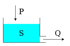
The single-element model is composed by a single reservoir that is governed by the following differential equation

\[\frac{\textrm{d}S}{\textrm{d}t}=P-Q\]

where \(S\) is the state of the reservoir, \(P\) is the precipitation input, and \(Q\) is the outflow, defined by the equation:

\[Q = kS^\alpha\]

where \(k\) and \(\alpha\) are parameters of the element. It can be noticed that, for simplicity, evapotranspiration is not considered in this demo.

The first step that needs to be done is initializing the numerical approximator, needed to construct the differential equation to solve, and the root finder used to find the value of the state that solves the approximation of the differential equation. In this case, we choose to use the Python implementation of implicit Euler (numerical approximator) and of the Pegasus algorithm (root finder). This can be done with the following code, where the default settings of the solver are used (refer to the solver docstring).

solver_python = PegasusPython()

approximator = ImplicitEulerPython(root_finder=solver_python)

After that, the element can be initialized

fast_reservoir = FastReservoir(
    parameters={'k': 0.01, 'alpha': 2.0},
    states={'S0': 10.0},
    approximation=approximator,
    id='FR'
)

During initialization, parameters (line 2) and initial state (line 3) are defined, together with the numerical approximator and the identifier (the identifier must be unique and cannot contain the character _).

After initialization, the time step used to solve the differential equation and the inputs of the element must be defined.

fast_reservoir.set_timestep(1.0)
fast_reservoir.set_input([precipitation])

Precipitation is a numpy array containing the precipitation time series. Note that the length of the simulation (i.e., number of time steps to run the model) cannot be defined and it is automatically set equal to the length of the input arrays.

At this point, the element can be run, calling the method get_output

output = fast_reservoir.get_output()[0]

The method will run the element for all the time steps solving the differential equation and return a list containing all the output arrays of the element (in this specific case there is only one output, \(Q\)).

After running, the state of the reservoir (for all the time steps) is saved in the state_array attribute of the element and can be inspected

reservoir_state = fast_reservoir.state_array[:, 0]

the state_array is a 2D array with as many row (first dimension) as the number of time steps and as many columns (second dimension) as the number of states. The order of the states is defined in the documentation of the element.

The plot shows the output of the simulation.

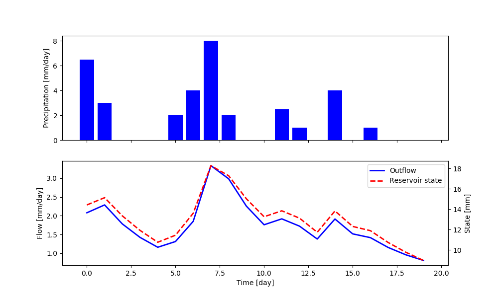
Note that the get_output method also sets the element states to their value at the final time step (in this case 8.98). Therefore, if the method is called again, it will use this value as initial state instead to the one defined at initialization. The states of the model can be reset calling the reset_states method.

fast_reservoir.reset_states()

Lumped model structure¶

We now move from a single-element configuration to multiple elements connected. For simplicity, we limit the complexity at two elements; more complex configurations can be found in the Application: implementation of existing conceptual models page.

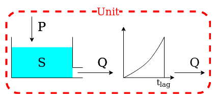
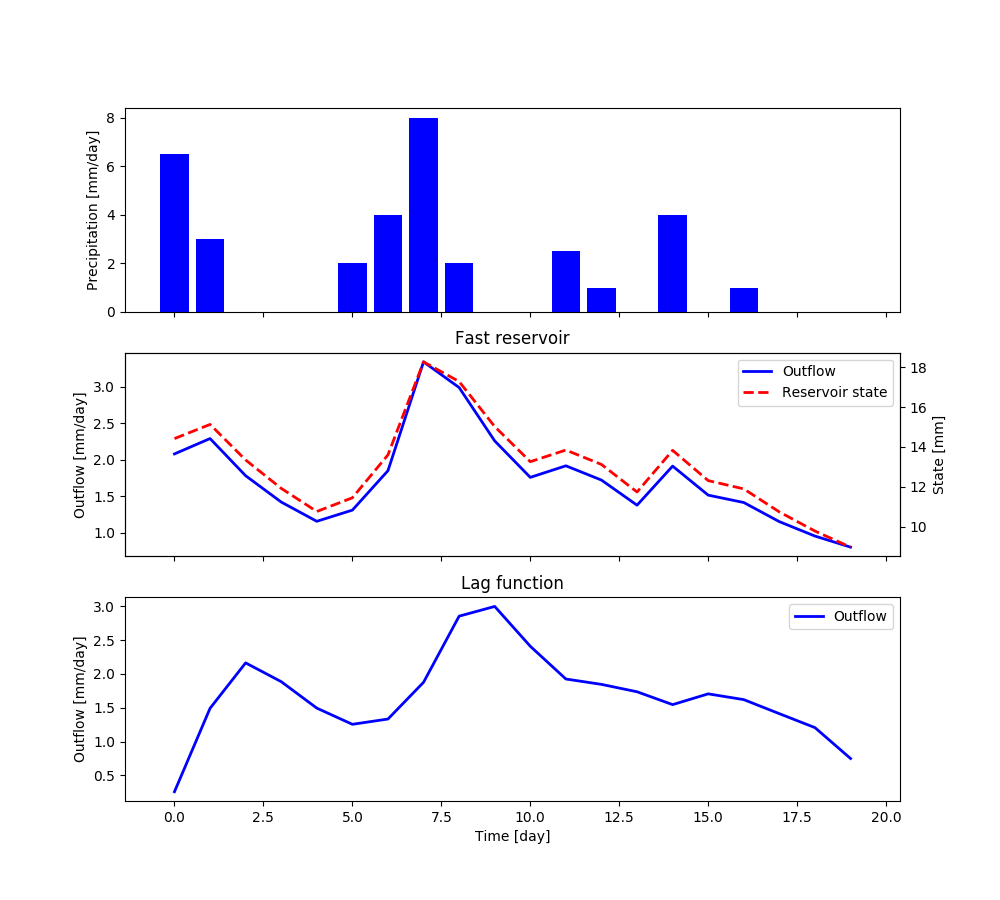
The structure is composed by a reservoir, which output is taken, as input, by a lag function. The lag function convolutes the incoming flux using the function

\[Q_{\textrm{out}}=Q_{\textrm{in}} \left(\frac{t}{t_{\textrm{lag}}}\right)^ {\frac{5}{2}} \qquad \textrm{for }t<t_{\textrm{lag}}\]

and its behavior is controlled by the parameter \(t_{\textrm{lag}}\).

The first step consists in initializing the two elements that compose the structure

fast_reservoir = FastReservoir(
    parameters={'k': 0.01, 'alpha': 2.0},
    states={'S0': 10.0},
    approximation=approximator,
    id='FR'
)

lag_function = UnitHydrograph1(
    parameters={'lag-time': 2.3},
    states={'lag': None},
    id='lag-fun'
)

Note that the initial state of the lag function has been set to None (line 10); in this case the element will initialize the state to an arrays of zeros of the proper length, depending on the value of \(t_{\textrm{lag}}\) (in this specific case, 3).

We can, then, initialize the unit that connect the elements, defining the model structure

unit_1 = Unit(
    layers=[[fast_reservoir], [lag_function]],
    id='unit-1'
)

Line 2 defines the structure; it is a 2D list where the inner level sets the elements belonging to each layer an the outer level lists the layers. Note that the order of the elements in the list is of primary importance. Refer to Unit for further details.

After initialization, time step and inputs must be defined

unit_1.set_timestep(1.0)
unit_1.set_input([precipitation])

The unit sets the time step of all the elements that contains to the provided value and transfers the inputs to the first element (the reservoir, in this example).

After that, the unit can be run

output = unit_1.get_output()[0]

The unit will call the get_output method of all its elements, from upstream to downstream, set the inputs of the downstream elements to the output of their respective upstream elements, and return the output of the last element.

The outputs and the states of the internal elements can be inspected after running the model

fr_state = unit_1.get_internal(id='FR', attribute='state_array')[:, 0]
fr_output = unit_1.call_internal(id='FR', method='get_output', solve=False)[0]

Note that (line 2) we need to pass to the function get_output of the reservoir the argument solve=False in order to avoid to re-run the element.

The plot shows the output of the simulation.

The elements of the unit can be re-set to their initial state

unit_1.reset_states()

Multiple units configuration¶

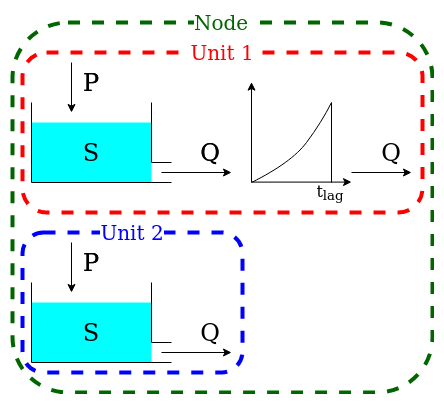
A catchment (node) can be composed by different areas that react differently to the same precipitation input. We may have 70% of the catchment that can be represented with the structure described in the previous section and 30% that can be described simply by a single reservoir.

This behavior can be simulated with SuperflexPy creating a node that contains multiple units.

The first step consists in initializing the two units and the elements composing them, as done in the previous sections.

fast_reservoir = FastReservoir(
    parameters={'k': 0.01, 'alpha': 2.0},
    states={'S0': 10.0},
    approximation=approximator,
    id='FR'
)

lag_function = UnitHydrograph1(
    parameters={'lag-time': 2.3},
    states={'lag': None},
    id='lag-fun'
)

unit_1 = Unit(
    layers=[[fast_reservoir], [lag_function]],
    id='unit-1'
)

unit_2 = Unit(
    layers=[[fast_reservoir]],
    id='unit-2'
)

Note that, once the elements are added to a unit, they become independent, meaning that any change to the reservoir contained in unit-1 does not affect the reservoir in unit-2.

At this point, the node can be initialized, putting together the two units

node_1 = Node(
    units=[unit_1, unit_2],
    weights=[0.7, 0.3],
    area=10.0,
    id='node-1'
)

Line 2 contains the list of the units that belong to the node, line 3 their weight (i.e. part of the node outflow influenced by this unit). The representative area of the node (line 4) will be used, in case, by the network.

After that, time step and inputs must be defined

node_1.set_timestep(1.0)
node_1.set_input([precipitation])

the same time step will be set to the elements composing all the units of the node, the inputs will be passed to all the units of the node.

We can now run the node and collect its output

output = node_1.get_output()[0]

The node will call the get_output method of all the units and aggregate their outputs using the weights. In the case of multiple fluxes (e.g., water and contaminants) their order must be the same in all the units.

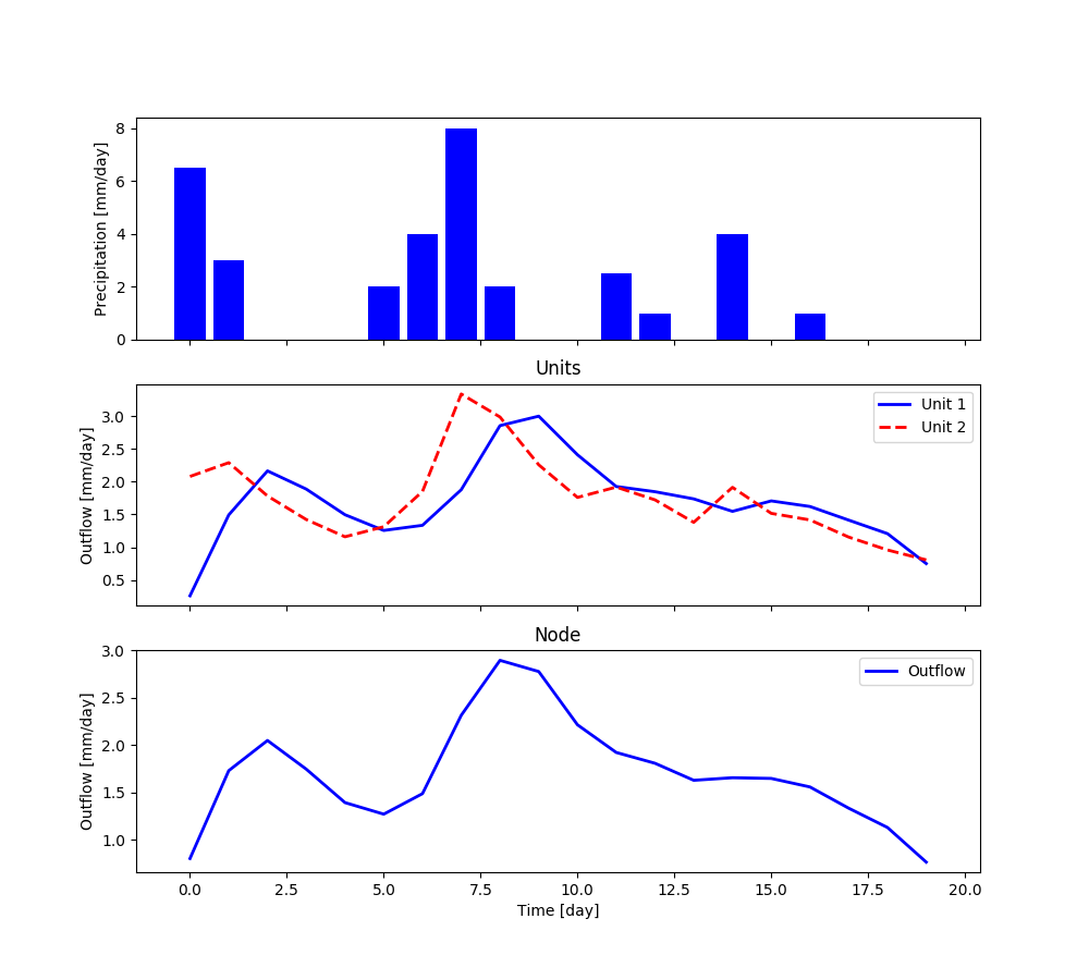
The outputs of the single units, as well as the states and fluxes of the elements composing them, can be inspected

output_unit_1 = node_1.call_internal(id='unit-1', method='get_output', solve=False)[0]
output_unit_2 = node_1.call_internal(id='unit-2', method='get_output', solve=False)[0]

The plot shows the output of the simulation.

All the elements composing the node can be re-set to their initial state

node_1.reset_states()

Multiple nodes in a network¶

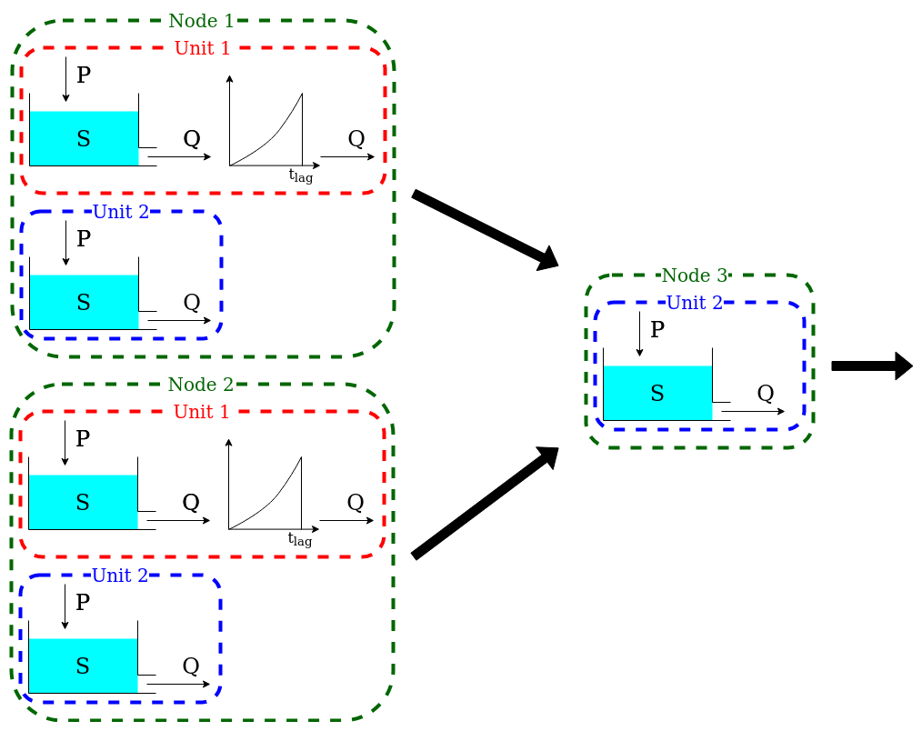
A watershed can be composed by several catchments connected in a network that have different inputs but share areas with the same hydrological behavior. This can be simulated with SuperflexPy creating a network that contains multiple nodes.

The first step for creating a network is initializing the nodes composing it.

fast_reservoir = FastReservoir(
    parameters={'k': 0.01, 'alpha': 2.0},
    states={'S0': 10.0},
    approximation=approximator,
    id='FR'
)

lag_function = UnitHydrograph1(
    parameters={'lag-time': 2.3},
    states={'lag': None},
    id='lag-fun'
)

unit_1 = Unit(
    layers=[[fast_reservoir], [lag_function]],
    id='unit-1'
)

unit_2 = Unit(
    layers=[[fast_reservoir]],
    id='unit-2'
)

node_1 = Node(
    units=[unit_1, unit_2],
    weights=[0.7, 0.3],
    area=10.0,
    id='node-1'
)

node_2 = Node(
    units=[unit_1, unit_2],
    weights=[0.3, 0.7],
    area=5.0,
    id='node-2'
)

node_3 = Node(
    units=[unit_2],
    weights=[1.0],
    area=3.0,
    id='node-3'
)

node-1 and node-2 contains both the units but with different proportions; node-3 contains only unit-2. When units are added to a catchment the states of the elements belonging to them remain independent while the parameters stay linked, meaning that the change of a parameter in unit-1 in node-1 is applied also in unit-1 in node-2. Different behavior can be achieve setting the parameter shared_parameters equal to False when initializing the nodes.

At this point, the network can be initialized

net = Network(
    nodes=[node_1, node_2, node_3],
    topography={
        'node-1': 'node-3',
        'node-2': 'node-3',
        'node-3': None
    }
)

Line 2 lists the nodes belonging to the network, lines 4-6 define the topology of the network; this is done with a dictionary that has the identifier of the nodes as key and the identifier of the single downstream node as value; the most downstream node has value None.

The inputs are catchment-specific and must be provided to each catchment, as done in the single-node case.

node_1.set_input([precipitation])
node_2.set_input([precipitation * 0.5])
node_3.set_input([precipitation + 1.0])

The time step is set by the network to the same value for all the nodes.

net.set_timestep(1.0)

We can now run the network and get the output values

output = net.get_output()

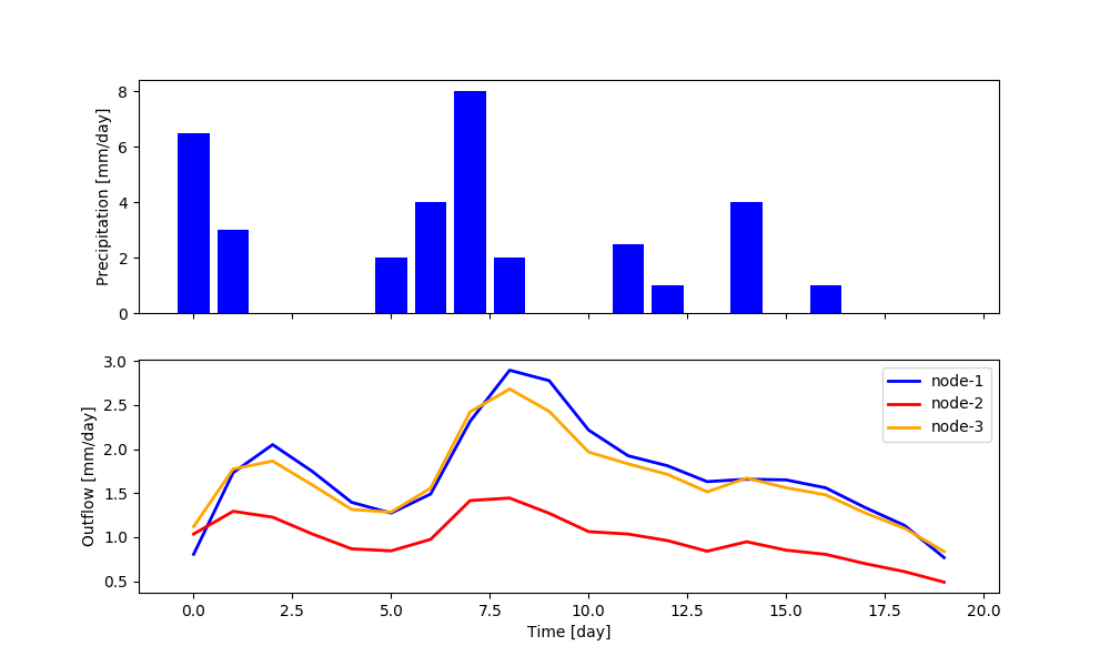
The network runs the nodes from upstream to downstream, collects their output, and route them to the outlet. The output of the network is a dictionary that has the identifier of the nodes, as key, and the list of output fluxes, as value. It is also possible to inspect the internals of the nodes, as done with the single-node case.

output_unit_1_node_1 = net.call_internal(id='node-1_unit-1',
                                         method='get_output',
                                         solve=False)[0]

The plot shows the results of the simulation.