Note
Last update 04/09/2020
Numerical routines for solving ODEs
Reservoirs are among the most common elements in conceptual hyrdological models. While their dynamic changes, reservoirs are still controlled by one (or more) ordinary differential equation (ODE) of the form
The analytical solution of such differential equation is almost always impossible to obtain and, therefore, a numerical approximation has to be constructed and solved.
In most of the cases, when a robust numerical approximation is used (e.g. Implicit Euler), the solution of the numerical approximation (i.e. finding a value of the state \(S\) that solves the algebraic equation) requires an iterative procedure, since an algebraic solution cannot be defined.
The solution of the ODE, therefore, can be seen as a two-steps approach:
- Find a numerical approximation of the ODE
- Solve such numerical approximation
This can be done in SuperflexPy using two components:
NumericalApproximator and RootFinder. The first uses the fluxes
from the reservoir element to construct a numerical approximation of the ODE,
the second finds, numerically, the root of such approximation.
SuperflexPy provides already two numerical approximators (implicit and explicit
Euler) and a root finder (which uses the Pegasus method). Other algorithms can
be used extending the classes NumericalApproximator and
RootFinder.
Numerical approximator
The implementation of a customized numerical approximator can be done extending
the class NumericalApproximator and implementing two methods:
_get_fluxes and _differential_equation.
1 2 3 4 5 6 7 8 9 10 11 12 13 14 15 | class CustomNumericalApproximator(NumericalApproximator):
@staticmethod
def _get_fluxes(fluxes, S, S0, args):
# Some code here
return fluxes
@staticmethod
def _differential_equation(fluxes, S, S0, dt, args, ind):
# Some code here
return [dif_eq, min_val, max_val]
|
where fluxes is a list of functions used to calculate the fluxes,
S is an array of states that solve the ODE for the different time
steps, S0 is the initial state, dt is the time step,
args is a list of additional arguments used by the functions in
fluxes, and ind is the index of the input arrays to use.
The first method (_get_fluxes) is responsible for calculating the fluxes
after the ODE has been solved and operates with a vector of states. The second
method (_differential_equation) calculates the approximation of the ODE
and it is designed to be interfaced to the root finder, returning the value of
the differential equation and the minimum and maximum boundary for the search of
the root.
To understand better how these methods work, please have a look at the
implementation of ImplicitEuler and ExplicitEuler.
Root finder
The implementation of a root finder can be done extending the class
RootFinder implementing the method solve.
1 2 3 4 5 6 7 | class CustomRootFinder(RootFinder):
def solve(self, dif_eq, fluxes, S0, dt, ind, args):
# Some code here
return root
|
where dif_eq is a function that calculates the value of the
approximated ODE, fluxes is a list of functions used to calculate
the fluxes, S0 is the initial state, dt is the time step,
args is a list of additional arguments used by the functions in
fluxes, and ind is the index of the input arrays to use.
The method solve is responsible for finding the numerical solution of
the approximated ODE.
To understand better how this method works, please have a look at the
implementation of Pegasus.
Computational efficiency with Numpy and Numba
Conceptual hydrological models are often associated to computationally demanding tasks, such as parameter calibration and uncertainty quantification, which require multiple model runs (even millions). Computational efficiency is therefore an important requirement of a SuperflexPy.
Computational efficiency is not the greatest strength of pure Python but libraries like Numpy and Numba can help in pushing the performance close to Fortran or C.
Numpy provides highly efficient arrays that can be transformed with C-time performance, as long as vector operations (i.e. elementwise operations between arrays) are run; Numba provides a “just-in-time compiler” that can be applied to a normal Python method to compile, at runtime, its content to machine code that interacts efficiently with NumPy arrays. This operation is extremely effective when solving ODEs where the method loops through a vector to perform some element-wise operations.
For this reason we provide a Numba-optimized version of the
NumericalApproximator and of the RootFinder that enables to
solve ODEs efficiently.
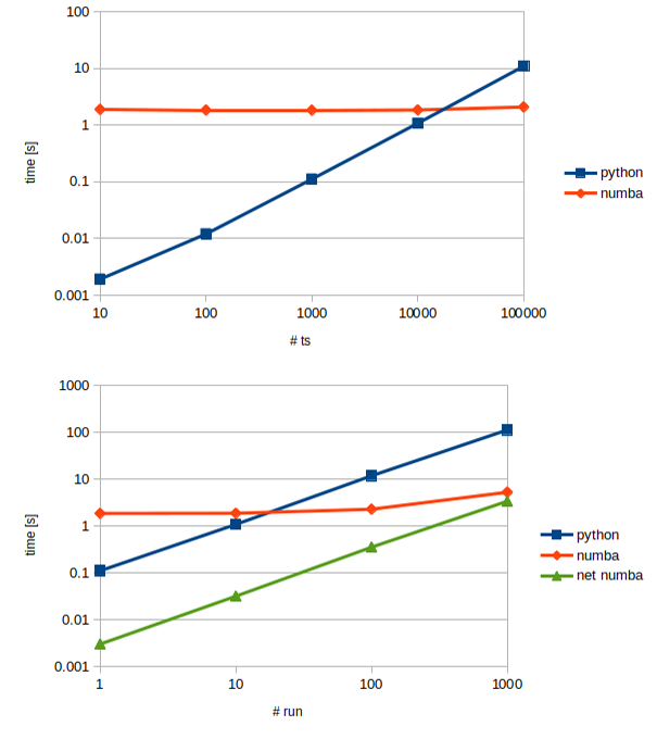
The figure shows the results of a benchmark that compares the execution times
of the pure Python vs. the Numba implementation, in relation to the length of
the time series (panel a) and to the number of model runs (panel b). The plots
clearly show the tradeoff between compile time (which is zero for Python and
around 2 seconds for Numba) and run time, where Numba is 30 times faster than
Python. This means that the choice of the implementation to use, which can be
done simply using a different NumericalApproximator implementation, may
depend on the application: a single run of the HYMOD model, with the
implicit Euler numerical solver and a time series of 1000 time steps takes 0.11
seconds with Python and 1.85 with Numba while, if the same model is run 100
times (for a calibration, for example) the Numba version takes 2.35 seconds
while the Python version 11.75 seconds.